Shapley Values
This is another blog post in the series on model explainability. Here I will provide a brief description of Shapley values in the context of explaining outputs of complex models. The concept of Shapley values originates from cooperative game theory, where it represents one of the possible solutions to a problem of splitting the total gain or loss from a cooperative game between the participating players that form a coalition. Wikipedia provides the following setup:
A coalition of players cooperates, and obtains a certain overall gain from that cooperation. Since some players may contribute more to the coalition than others or may possess different bargaining power (for example threatening to destroy the whole surplus), what final distribution of generated surplus among the players should arise in any particular game? Or phrased differently: how important is each player to the overall cooperation, and what payoff can he or she reasonably expect? The Shapley value provides one possible answer to this question.
As an example of a cooperative game, consider a government that needs to maintain the support of the majority of members of parliament (MPs) to stay in power. For simplicity, let’s assume that there are three political parties A, B and C with the membership counts shown in Figure 1.
Figure 1. Political Party Membership
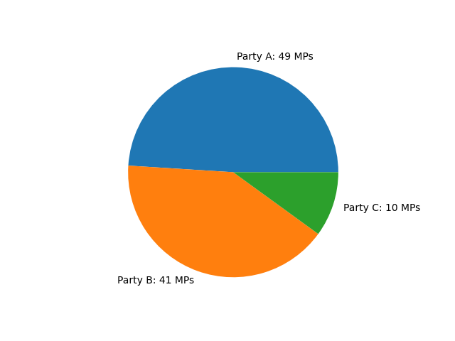
There are 100 MPs in total. Therefore, the government requires support from at least 51 MPs to stay in power. Since the largest party (A) has only 49 MPs, none of the parties can provide the required support on its own. Therefore, some cooperation between the political parties is necessary. In particular, majority support can be provided by any of the following coalitions:
- party A and party B: 90 members;
- party A and party C: 59 members;
- party B and party C: 51 members;
- party A, party B and party C: 100 members.
Now the question is: Assuming that providing the majority support for the government is associated with a reward of 1, what share of that reward should be attributed to each party? Is it fair to associate with each party a reward proportional to how many MPs belong to that party? If we are to do this, party C would only get a value of 0.1. However, party C is in three out of four majority coalitions. Therefore, its actual political power appears to be higher than what party membership predicts. This is where the concept of Shapley values can be used.
Let us formulate the problem mathematically. We have a set $N$ of players, $|N|=n$, and a characteristic function $v: 2^N\rightarrow \mathbb{R}, v(\emptyset)=0$. Let $S\subset N$ be any coalition of players. Then $v(S)$ can be interpreted as the worth of the coalition, i.e., the total expected payoff that the players in the coalition can obtain by cooperating. With that, the amount that player $i$ is given in a coalition game $(v, N)$ is
\[\begin{equation} \label{eq: shap} \varphi_i = \sum_{S\subset N\backslash \{i\}} \frac{|S|!\left(n - |S| - 1 \right)!}{n!} \times \left(v\left(S\cup \{i\}\right) - v\left(S\right)\right), \end{equation}\]where
- $S\subset N\backslash {i}$ is any coalition without player $i$;
- $v\left(S\right)$ is worth of coalition $S$;
- $v\left(S\cup {i}\right)$ is worth of coalition $S$ with the addition of player $i$;
- $v\left(S\cup {i}\right) - v\left(S\right)$ is the marginal contribution of player $i$ to coalition $S$.
Therefore, the above formula says that the worth of player $i$ is equal to the average marginal contribution that this player provides to each of the coalitions.
Using formula ($\ref{eq: shap}$), we can estimate the worth of party C in our example as follows:
\[\begin{align*} \varphi_3 &= \frac{|\emptyset|!(3 - |\emptyset| - 1)!}{3!} \times \left(v(\emptyset \cup\{3\}) - v(\emptyset)\right) + \frac{|\{1\}|!(3 - |\{1\}| - 1)!}{3!} \times \left(v(\{1\} \cup\{3\}) - v(\{1\})\right) + \frac{|\{2\}|!(3 - |\{2\}| - 1)!}{3!} \times \left(v(\{2\} \cup\{3\}) - v(\{2\})\right) + \frac{|\{1, 2\}|!(3 - |\{1, 2\}| - 1)!}{3!} \times \left(v(\{1, 2\} \cup\{3\}) - v(\{1, 2\})\right) \\ &= \frac{1}{3}\times (0 - 0) + \frac{1}{6} \times (1 - 0) + \frac{1}{6}\times (1 - 0) + \frac{1}{3} \times (1 - 1) \\ &= \frac{1}{3}. \end{align*}\]Thus, even though party C has only 10 MPs, it wields a third of all political power. Actually, if we were to repeat the above calculations for parties A and B, we would get the same results, i.e., that each is worth a third. It turns out that in this particular case all parties have the same political influence. This should not surprise us given that none of the parties can provide majority on their own and every party needs to join a coalition with at least one other party to form a majority.
Shapley Values for Explaining Model Outputs
Now that we have introduced the concept of Shapley values, how can we apply it in the domain of model output explanation? What is the game and who are the players? Let us introduce the following notation:
- $f: \mathbb{R}^d \rightarrow \mathbb{R}$ is a trained model;
- $f(\textbf{x}), \textbf{x} \in \mathbb{R}^d$, is the output from the model that we want to explain.
Then the players are the different feature values in the input feature vector $\textbf{x}$. These “players” are in a coalition to produce $f(\textbf{x})$. The total gain or loss from the game is the difference between $f(\textbf{x})$ and the average prediction. In practice, the latter can be estimated as
\[\begin{equation*} \frac{1}{N}\sum_{i\in T}f(\textbf{x}_i), \end{equation*}\]where $T, |T| = N$, is the set of training indices.
What is a coalition of players in this settings and how do we estimate its worth? The worth of a coalition of features is the difference between the output of the model where only features in the coalition retain their values and the effects of the remaining features are averaged out (for example, by substituting the values from the training dataset), and the average prediction. It will all become more clear in the next section where we implement Shapley value estimation in Python.
Python Implementation
We will require the following Python libraries.
import numpy as np
import pandas as pd
import matplotlib.pyplot as plt

from sklearn.base import BaseEstimator
from sklearn.ensemble import RandomForestRegressor
from sklearn.model_selection import train_test_split

from ucimlrepo import fetch_ucirepo

from itertools import chain, combinations
import math
from typing import List, Union, Optional
In the previous blog posts on model explainability (Local Interpretable Model-Agnostic Explanations, Partial Dependence Plots and Permutation Feature Importance) we worked with the Heart Failure Clinical Records dataset. That dataset had 12 features. As per equation (\ref{eq: shap}), estimating Shapley values requires investigating all possible coalitions of players (features). Thus, the computational costs are rising very sharply with the number of features. Therefore, we will work with Liver Disorders dataset that has five features and is also available from the UCI Irvine Machine Learning Repository. Below we load the dataset.
liver_disorders = fetch_ucirepo(id=60)

X = liver_disorders.data.features
y = liver_disorders.data.targets.values.flatten()

print(f"Dataset shape: {X.shape}")
Dataset shape: (345, 5)
The dataset contains 345 observations and the following five features:
mcv: mean corpuscular volume;alkphos: alkaline phosphotase;sgpt: alanine aminotransferase;sgot: aspartate aminotransferase;gammagt: gamma-glutamyl transpeptidase.
According to the dataset description, “The first 5 variables are all blood tests which are thought to be sensitive to liver disorders that might arise from excessive alcohol consumption. Each line in the dataset constitutes the record of a single male individual.”
Below we provide a summary of the dataset.
def describe_df(df: pd.DataFrame) -> pd.DataFrame:
    """
    Describe pandas dataframe.

    :param df: input dataframe
    :return: description of the dataset
    """
    col_types = df.dtypes
    col_types.name = "dtype"

    n_missing = df.isna().astype(int).sum(axis=0)
    n_missing.name = "n_missing"

    pct_missing = n_missing / len(df)
    pct_missing.name = "pct_missing"

    n_unique = df.nunique()
    n_unique.name = "n_unique"

    skewness = df.skew()
    skewness.name = "skewness"

    kurtosis = df.kurt()
    kurtosis.name = "kurtosis"

    return pd.concat([col_types, n_missing, pct_missing, n_unique, df.describe().T, skewness, kurtosis],
                     axis=1)

describe_df(X)
| dtype | n_missing | pct_missing | n_unique | count | mean | std | min | 25% | 50% | 75% | max | skewness | kurtosis | |
|---|---|---|---|---|---|---|---|---|---|---|---|---|---|---|
| mcv | int64 | 0 | 0.0 | 26 | 345.0 | 90.159420 | 4.448096 | 65.0 | 87.0 | 90.0 | 93.0 | 103.0 | -0.388433 | 2.584958 |
| alkphos | int64 | 0 | 0.0 | 78 | 345.0 | 69.869565 | 18.347670 | 23.0 | 57.0 | 67.0 | 80.0 | 138.0 | 0.753667 | 0.747883 |
| sgpt | int64 | 0 | 0.0 | 67 | 345.0 | 30.405797 | 19.512309 | 4.0 | 19.0 | 26.0 | 34.0 | 155.0 | 3.063499 | 13.813912 |
| sgot | int64 | 0 | 0.0 | 47 | 345.0 | 24.643478 | 10.064494 | 5.0 | 19.0 | 23.0 | 27.0 | 82.0 | 2.293072 | 8.140165 |
| gammagt | int64 | 0 | 0.0 | 94 | 345.0 | 38.284058 | 39.254616 | 5.0 | 15.0 | 25.0 | 46.0 | 297.0 | 2.866094 | 10.476749 |
We note the following:
- there are no missing values;
- all features are of integer type;
- all features take on positive values.
The target is the number of half-pint equivalents of alcoholic beverages drunk per day. Thus, this is a regression type problem.
We will split the whole dataset into training and test subsets with the proportion of training observations equal to 0.8.
X_train, X_test, y_train, y_test = train_test_split(X, y, test_size=0.2, random_state=4)
Next we fit random forest regressor.
estimator = RandomForestRegressor(
    n_estimators=28,
    max_depth=4,
    min_samples_split=0.16,
    min_samples_leaf=0.024,
    max_features='sqrt',
    random_state=4
)
estimator.fit(X_train, y_train)

train_r2 = estimator.score(X_train, y_train)
test_r2 = estimator.score(X_test, y_test)
print(f"R-squared (train): {round(train_r2, 4)}")
print(f"R-squared (test): {round(test_r2, 4)}")
R-squared (train): 0.2537
R-squared (test): 0.2509
Without any loss of generality, let us investigate the first patient in the test set.
X_test.iloc[0]
mcv        91
alkphos    52
sgpt       15
sgot       22
gammagt    11
Name: 63, dtype: int64
round(estimator.predict(X_test.iloc[0].values.reshape(1, -1))[0], 4)
2.5006
According to the model, these blood test results imply that the patient drank 2.5 half-pint equivalents of alcoholic beverages per day. While the average across the whole training sample is equal to 3.4591.
round(np.average(estimator.predict(X_train)), 4)
3.4591
Therefore, the difference between the prediction for this patient and the average prediction is equal to $2.5006 - 3.4591 = -0.9585$. Now we are interested in how the blood test results of this patient explain the difference. This is where Shapley values come into play. Below we provide implementation of explain_obs_shap function that will provide one way of answering this question.
def explain_obs_shap(estimator: BaseEstimator,
                     obs: Union[np.ndarray, pd.Series, pd.DataFrame],
                     X: Union[np.ndarray, pd.DataFrame],
                     names: Optional[List[str]]=None,
                     digits: int=4):
    """
    Provide Shapley explanations for `obs`.

    :param estimator: estimator that has been fit to data
    :param obs: observation to explain of shape (1, n_features)
    :param X: features of shape (n_obs, n_features)
    :param names: feature names that correspond to features in `X`
    :param digits: number of decimals to use when rounding the number
    :return: Shapley explanation of `obs`
    """
    if isinstance(obs, (pd.Series, pd.DataFrame)):
        obs = obs.values
    obs = obs.reshape(1, -1)

    if names is not None:
        if X.shape[1] != len(names):
            raise RuntimeError(f"`names` must correspond to features in `X`.")
    else:
        if isinstance(X, pd.DataFrame):
            names = X.columns
        else:
            names = list(range(X.shape[1]))

    feature_contributions = {}
    for i, feature in enumerate(names):
        feature_contributions[feature] = round(
            feature_val_shap(
                estimator=estimator,
                obs=obs,
                X=X,
                feature=i
            ),
            digits
        )

    return feature_contributions


def feature_val_shap(estimator: BaseEstimator,
                     obs: Union[np.ndarray, pd.DataFrame],
                     X: Union[np.ndarray, pd.DataFrame],
                     feature: int) -> float:
    """
    Estimate Shapley value for a given feature.

    :param estimator: estimator that has been fit to data
    :param obs: observation to explain of shape (1, n_features)
    :param X: features of shape (n_obs, n_features)
    :param feature: index of feature to explain
    :return: Shapley value for `feature`
    """
    s = 0
    n = X.shape[1]
    for mask in _generate_feature_masks(X.shape[1] - 1):
        w = (math.factorial(np.sum(mask)) * math.factorial(n - np.sum(mask)  - 1)) / math.factorial(n)
        s += w * (np.average(estimator.predict(_update_features(obs, X, np.insert(mask, feature, 1)))) - np.average(estimator.predict(_update_features(obs, X, np.insert(mask, feature, 0)))))
    return s


def _generate_feature_masks(n: int) -> np.ndarray:
    """
    Generate feature masks.

    :param n: number of features
    :return: 2-d numpy array where each row is a separate feature mask
    """
    subset_masks = np.zeros((2**n, n)).astype(int)
    for i, subset in enumerate(chain.from_iterable(combinations(range(n), r) for r in range(1, n + 1))):
        subset_masks[i + 1, subset] = 1
    return subset_masks


def _update_features(obs: Union[np.ndarray, pd.DataFrame],
                     X: Union[np.ndarray, pd.DataFrame],
                     mask: np.ndarray) -> Union[np.ndarray, pd.DataFrame]:
    """
    Update input features by replacing feature values with values from `obs` whenever
    mask is equal to 1 for that particular feature.

    :param obs: observation to explain of shape (1, n_features)
    :param X: features of shape (n_obs, n_features)
    :param mask: feature mask
    :return: updated features
    """
    _X = X.copy()
    for i in range(len(mask)):
        if mask[i] == 1:
            if isinstance(X, pd.DataFrame):
                _X.iloc[:, i] = obs[0, i]
            else:
                _X[:, i] = obs[0, i]
    return _X
Let us apply explain_obs_shap function to the patient.
expl = explain_obs_shap(
    estimator=estimator,
    obs=X_test.iloc[0],
    X=X_train,
    names=X_train.columns)
expl
{'mcv': -0.0241,
 'alkphos': 0.0434,
 'sgpt': 0.0845,
 'sgot': -0.1341,
 'gammagt': -0.9282}
The Shapley value analysis reveals that gammagt is the feature most responsible for the lower than average model output for this patient. According to the Cleveland Clinic page on Gamma-Glutamyl Transferase (GGT) Test,
A gamma-glutamyl transferase (GGT) blood test measures the activity of GGT in your blood. GGT may leak into your bloodstream if your liver or bile duct is damaged, so having high levels of GGT in your blood may indicate liver disease or damage to your liver’s bile ducts. Bile ducts are tubes that carry bile (a fluid that’s important for digestion) in and out of your liver.
Your GGT levels can also rise from administration of foreign substances such as medications (like phenobarbital, phenytoin or warfarin) or alcohol.
We can check how this patient’s gammagt feature compares with the average across the whole training sample.
print(f"gammagt (patient): {X_test.iloc[0]['gammagt']}")
print(f"gammagt (average): {round(X_train.gammagt.mean(), 4)}")
gammagt (patient): 11
gammagt (average): 37.6268
It is indeed the case that the patient has lower than average gammagt.
Note that the sum of the feature contributions from the Shapley analysis will be exactly equal to the difference between the output for this patient and the average prediction, i.e,
\[\begin{equation*} -0.0241 + 0.0434 + 0.0845 - 0.1341 - 0.9282 = -0.9585. \end{equation*}\]Now that we know how to interpret the Shapley values, let us explain how explain_obs_shap function works. Let us first look into _generate_feature_masks auxiliary function.
def _generate_feature_masks(n: int) -> np.ndarray:
    """
    Generate feature masks.

    :param n: number of features
    :return: 2-d numpy array where each row is a separate feature mask
    """
    subset_masks = np.zeros((2**n, n)).astype(int)
    for i, subset in enumerate(chain.from_iterable(combinations(range(n), r) for r in range(1, n + 1))):
        subset_masks[i + 1, subset] = 1
    return subset_masks
This function uses a single parameter n that represents number of features. It outputs an array of feature masks where each mask shows which features are present and which are absent. For example, if n is equal to 3, we will get the following masks.
_generate_feature_masks(3)
array([[0, 0, 0],
       [1, 0, 0],
       [0, 1, 0],
       [0, 0, 1],
       [1, 1, 0],
       [1, 0, 1],
       [0, 1, 1],
       [1, 1, 1]])
This function basically finds all the possible coalitions of $n$ features in equation ($\ref{eq: shap}$).
The next auxiliary function is _update_features.
def _update_features(obs: Union[np.ndarray, pd.DataFrame],
                     X: Union[np.ndarray, pd.DataFrame],
                     mask: np.ndarray) -> Union[np.ndarray, pd.DataFrame]:
    """
    Update input features by replacing feature values with values from `obs` whenever
    mask is equal to 1 for that particular feature.

    :param obs: observation to explain of shape (1, n_features)
    :param X: features of shape (n_obs, n_features)
    :param mask: feature mask
    :return: updated features
    """
    _X = X.copy()
    for i in range(len(mask)):
        if mask[i] == 1:
            if isinstance(X, pd.DataFrame):
                _X.iloc[:, i] = obs[0, i]
            else:
                _X[:, i] = obs[0, i]
    return _X
This function updates feature values in X as follows: if a given feature is associated with a value of 1 in mask, then replace its values with the value for that feature in obs.
Finally, feature_val_shap is the implementation of equation ($\ref{eq: shap}$) and it estimates Shapley value of a given feature.