Permutation Feature Importance
Investigating feature importances for a developed model is a very important step in achieving the goal of interpretable machine learning. This not only allows to confirm that the important features have been picked up by the model but also to catch leakages in developed pipelines when, for example, unimportant (or even random) features happen to have significant predictive power. One model-agnostic approach is permutation feature importance. The approach works by measuring the importance of a given feature by observing by how much the performance of the model drops with respect to the metric of choice when this feature is randomly shuffled in the dataset. The larger the drop in the performance of the model, the more important the feature.
The algorithm to estimate permutation importance of a given feature can be described as follows:
- Estimate baseline model performance on a dataset, $P_b$;
- For each $i\in {1, 2, …, N}$ do:
- Permute the feature in the dataset;
- Estimate the resulting model performance, $P_{i}$;
- Estimate importance of the feature as the mean decrease in model performance:
As with any statistical method, there are certain underlying assumptions:
- one needs to be careful when investigating importance of a feature that is highly correlated with other features in the dataset: the true decrease in the model’s performance may be masked by the presence of correlated features in which case the feature may appear more or less important than it actually is;
- the model possesses predictive power for the task under consideration. Important feature for a bad model is not necessarily important for a good model;
- permutation feature importances depend on the chosen measure of model performance, i.e., relative feature importances may differ for the same estimator instance if different measures of model performance are used;
- permutation feature importances depend on the chosen modeling approach. This means that different prediction algorithms may not agree on the relative importances of the features.
In the next section we will implement the algorithm in Python and test it on an actual dataset.
Python implementation
We begin by loading the required libraries.
import numpy as np
np.random.seed(4)
import pandas as pd
import matplotlib.pyplot as plt
import seaborn as sns
from sklearn.ensemble import RandomForestClassifier
from sklearn.linear_model import LogisticRegression
from sklearn.metrics import roc_auc_score
from sklearn.base import BaseEstimator, is_classifier
from sklearn.utils.validation import check_is_fitted
from sklearn.exceptions import NotFittedError
from typing import List, Optional, Callable, Union
Below we define permutation_feature_importance function that implements the permutation feature importance algorithm.
def permutation_feature_importance(estimator: BaseEstimator,
                                   X: pd.DataFrame,
                                   y: Union[pd.Series, np.ndarray],
                                   N: int=30,
                                   features: Optional[List[str]]=None,
                                   metric: Optional[Callable[[Union[pd.Series, np.ndarray], Union[pd.Series, np.ndarray]], float]]=None,
                                   use_proba: bool=False,
                                   mode: str="max",
                                   random_seed: Optional[int]=None) -> pd.DataFrame:
    """
    Estimate permutation feature importances.

    :param estimator: estimator that has been fit to data
    :param X: dataframe of features with shape (N_samples, N_features)
    :param y: true labels
    :param N: number of times to permute each feature
    :param features: list of features for which to estimate importances
    :param metric: custom metric
    :param use_proba: if True, use probabilities of positive class instead of class predictions
    :param mode: if "max", higher values of `metric` are associated with better performance
    :param random_seed: random seed for reproducibility
    """
    _check_estimator(estimator)
    if N < 1 or not isinstance(N, int):
        raise ValueError("Parameter `N` should be a positive integer.")
    if features:
        for feature in features:
            assert feature in X.columns, f"'{feature}' could not be found in the columns of the dataframe."
    else:
        features = list(X.columns)

    if mode not in ("max", "min"):
        raise ValueError("Parameter `mode` should be in ['max', 'min'].")
    multiplier = 1 if mode == "max" else -1

    if random_seed:
        np.random.seed(random_seed)

    if metric is None:
        baseline_score = estimator.score(X.values, y)
    else:
        preds = estimator.predict_proba(X.values)[:, 1] if use_proba else estimator.predict(X.values)
        baseline_score = metric(y, preds)

    res = pd.DataFrame(index=features, columns=["mean", "std"])

    for feature in features:
        score_changes = []
        for i in range(N):
            X_copy = X.copy()
            X_copy[feature] = np.random.permutation(X_copy[feature])
            if metric is None:
                permuted_score = estimator.score(X_copy.values, y)
            else:
                preds = estimator.predict_proba(X_copy.values)[:, 1] if use_proba else estimator.predict(X_copy.values)
                permuted_score = metric(y, preds)
            score_changes.append((baseline_score - permuted_score) * multiplier)
        res.loc[feature] = [np.mean(score_changes), np.std(score_changes)]
    res.reset_index(names="features", inplace=True)
    res.sort_values(["mean"], ascending=False, inplace=True)
    return res


def _check_estimator(estimator: BaseEstimator) -> None:
    """
    Check if estimator has been fit to data and has required methods.

    :param estimator: estimator to check
    """
    assert isinstance(estimator, BaseEstimator), "Estimator is not an instance of `BaseEstimator`."

    try:
        check_is_fitted(estimator)
    except NotFittedError:
        print("The estimator has not been fit to data. Please, fit the estimator to data first.")
Continuing with the theme of model explainability, we will use the heart failure clinical records dataset that can be downloaded from UC Irvine Machine Learning Repository. Let us load the dataset as pandas dataframe.
df = pd.read_csv("data/heart_failure_clinical_records_dataset.csv")
print(f"Dataset shape: {df.shape}")
df.head()
Dataset shape: (299, 13)
| age | anaemia | creatinine_phosphokinase | diabetes | ejection_fraction | high_blood_pressure | platelets | serum_creatinine | serum_sodium | sex | smoking | time | DEATH_EVENT | |
|---|---|---|---|---|---|---|---|---|---|---|---|---|---|
| 0 | 75.0 | 0 | 582 | 0 | 20 | 1 | 265000.00 | 1.9 | 130 | 1 | 0 | 4 | 1 |
| 1 | 55.0 | 0 | 7861 | 0 | 38 | 0 | 263358.03 | 1.1 | 136 | 1 | 0 | 6 | 1 |
| 2 | 65.0 | 0 | 146 | 0 | 20 | 0 | 162000.00 | 1.3 | 129 | 1 | 1 | 7 | 1 |
| 3 | 50.0 | 1 | 111 | 0 | 20 | 0 | 210000.00 | 1.9 | 137 | 1 | 0 | 7 | 1 |
| 4 | 65.0 | 1 | 160 | 1 | 20 | 0 | 327000.00 | 2.7 | 116 | 0 | 0 | 8 | 1 |
We have already performed exploratory data analysis of this dataset in the previous post on partial dependence plots. Therefore, we will just provide a summary statistics table below but will not spend time discussing the dataset.
def describe_df(df: pd.DataFrame) -> pd.DataFrame:
    """
    Describe pandas dataframe.

    :param df: input dataframe
    :return: description of the dataset
    """
    col_types = df.dtypes
    col_types.name = "dtype"

    n_missing = df.isna().astype(int).sum(axis=0)
    n_missing.name = "n_missing"

    pct_missing = n_missing / len(df)
    pct_missing.name = "pct_missing"

    n_unique = df.nunique()
    n_unique.name = "n_unique"

    skewness = df.skew()
    skewness.name = "skewness"

    kurtosis = df.kurt()
    kurtosis.name = "kurtosis"

    return pd.concat([col_types, n_missing, pct_missing, n_unique, df.describe().T, skewness, kurtosis],
                     axis=1)

describe_df(df)
| dtype | n_missing | pct_missing | n_unique | count | mean | std | min | 25% | 50% | 75% | max | skewness | kurtosis | |
|---|---|---|---|---|---|---|---|---|---|---|---|---|---|---|
| age | float64 | 0 | 0.0 | 47 | 299.0 | 60.833893 | 11.894809 | 40.0 | 51.0 | 60.0 | 70.0 | 95.0 | 0.423062 | -0.184871 |
| anaemia | int64 | 0 | 0.0 | 2 | 299.0 | 0.431438 | 0.496107 | 0.0 | 0.0 | 0.0 | 1.0 | 1.0 | 0.278261 | -1.935563 |
| creatinine_phosphokinase | int64 | 0 | 0.0 | 208 | 299.0 | 581.839465 | 970.287881 | 23.0 | 116.5 | 250.0 | 582.0 | 7861.0 | 4.463110 | 25.149046 |
| diabetes | int64 | 0 | 0.0 | 2 | 299.0 | 0.418060 | 0.494067 | 0.0 | 0.0 | 0.0 | 1.0 | 1.0 | 0.333929 | -1.901254 |
| ejection_fraction | int64 | 0 | 0.0 | 17 | 299.0 | 38.083612 | 11.834841 | 14.0 | 30.0 | 38.0 | 45.0 | 80.0 | 0.555383 | 0.041409 |
| high_blood_pressure | int64 | 0 | 0.0 | 2 | 299.0 | 0.351171 | 0.478136 | 0.0 | 0.0 | 0.0 | 1.0 | 1.0 | 0.626732 | -1.618076 |
| platelets | float64 | 0 | 0.0 | 176 | 299.0 | 263358.029264 | 97804.236869 | 25100.0 | 212500.0 | 262000.0 | 303500.0 | 850000.0 | 1.462321 | 6.209255 |
| serum_creatinine | float64 | 0 | 0.0 | 40 | 299.0 | 1.393880 | 1.034510 | 0.5 | 0.9 | 1.1 | 1.4 | 9.4 | 4.455996 | 25.828239 |
| serum_sodium | int64 | 0 | 0.0 | 27 | 299.0 | 136.625418 | 4.412477 | 113.0 | 134.0 | 137.0 | 140.0 | 148.0 | -1.048136 | 4.119712 |
| sex | int64 | 0 | 0.0 | 2 | 299.0 | 0.648829 | 0.478136 | 0.0 | 0.0 | 1.0 | 1.0 | 1.0 | -0.626732 | -1.618076 |
| smoking | int64 | 0 | 0.0 | 2 | 299.0 | 0.321070 | 0.467670 | 0.0 | 0.0 | 0.0 | 1.0 | 1.0 | 0.770349 | -1.416080 |
| time | int64 | 0 | 0.0 | 148 | 299.0 | 130.260870 | 77.614208 | 4.0 | 73.0 | 115.0 | 203.0 | 285.0 | 0.127803 | -1.212048 |
| DEATH_EVENT | int64 | 0 | 0.0 | 2 | 299.0 | 0.321070 | 0.467670 | 0.0 | 0.0 | 0.0 | 1.0 | 1.0 | 0.770349 | -1.416080 |
We will introduce a random feature to the dataset. This is done to show how a random feature may appear to have predictive power if there were issues with the model development process. In this case we will train a random forest algorithm (which can be considered as a relatively high-capacity algorithm for the dataset under consideration) on the whole dataset thereby introducing overfitting.
df["rand_feature"] = np.random.normal(0, 1, (df.shape[0]))

target = "DEATH_EVENT"
features = [col for col in df.columns if col not in ["time", target]]
Below we fit the algorithm on the whole dataset.
estimator = RandomForestClassifier(random_state=4)
X, y = df[features].values, df[target].values
estimator.fit(X, y);
Before estimating permutation feature importances we need to make sure that the model possess predictive power. By default, permutation_feature_importance function relies on the estimator’s score method. For random forest algorithm of sklearn it is mean accuracy. We will also check AUROC metric that is a very common metric for binary classification tasks.
print(f"Mean accuracy: {estimator.score(X, y)}")
print(f"AUROC: {roc_auc_score(y, estimator.predict_proba(X)[:, 1])}")
Mean accuracy: 1.0
AUROC: 0.9999999999999999
The model achieved the highest possible values on both metrics. This also means that the model is clearly overfit to the dataset.
Let us now check permutation feature importances using the default accuracy metric.
importances = permutation_feature_importance(estimator, df[features], y, random_seed=4)
sns.barplot(importances, x="mean", y="features")
plt.xlabel("Feature importance")
plt.ylabel("")
plt.title("Accuracy-based Permutation Feature Importances");
Figure 1. Accuracy-based Permutation Feature Importances. Random Forest
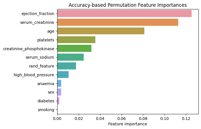
As can be seen from Figure 1, the two most important features for predicting death following a heart failure event are “ejection_fraction” and “serum_creatinine”. At the same time “smoking” appears to have no importance whatsoever. The random feature that we introduced appears near the middle and is more important than “high_blood_pressure” and “anaemia” explanatory variables. To verify that the obtained feature importances are reasonable, we compare them with the feature importances reported in “Machine learning can predict survival of patients with heart failure from serum creatinine and ejection fraction alone” by Chicco and Jurman (2020).
Figure 2. Random Forest Feature Selection
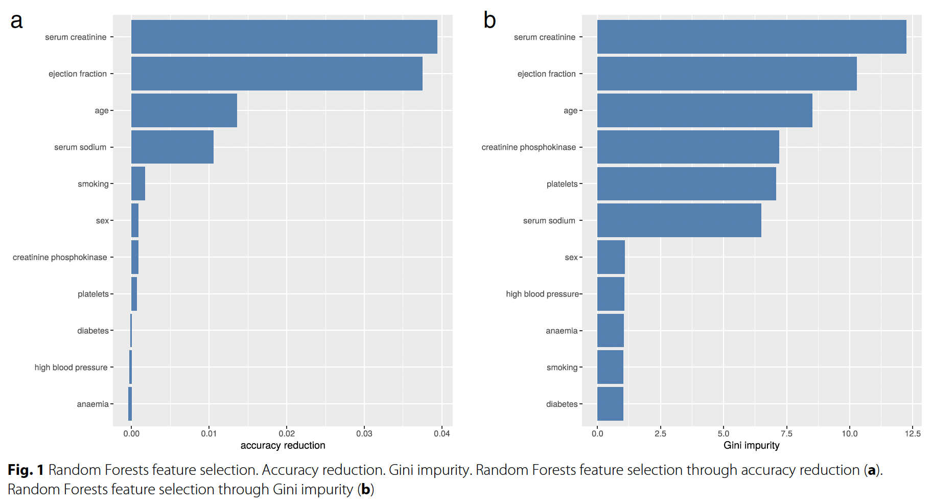
By comparing the permutation feature importances (Figure 1) with the feature importances based on accuracy reduction and gini impurity as reported by the authors of the paper (Figure 2), we can see they mostly align with some disagreements. This confirms that the obtained permutation feature importances are reasonable.
We continue by estimating permutation feature importances using AUROC as the metric.
importances = permutation_feature_importance(estimator,
                                             df[features], y,
                                             metric=roc_auc_score,
                                             use_proba=True,
                                             random_seed=4)
sns.barplot(importances, x="mean", y="features")
plt.xlabel("Feature importance")
plt.ylabel("")
plt.title("AUROC-based Permutation Feature Importances");
Figure 3. AUROC-based Permutation Feature Importances. Random Forest
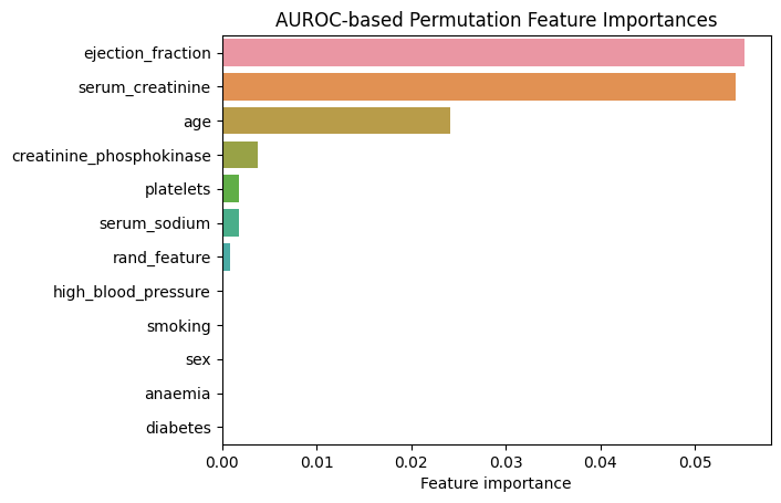
We can see that changing the metric resulted in changes in the relative importances of the features. As such, “platelets” is now less important than “creatinine_phosphokinase”. Also, some features completely “lost their importance”: “diabetes”, “anaemia”, “sex” and “high_blood_pressure”.
Finally, to show that permutation feature importances are dependent on the chosen modeling approach, we will fit logistic regression to the same dataset and estimate the resulting permutation feature importances.
estimator_log_r = LogisticRegression(random_state=4)
estimator_log_r.fit(X, y);
print(f"Mean accuracy: {estimator_log_r.score(X, y)}")
print(f"AUROC: {roc_auc_score(y, estimator_log_r.predict_proba(X)[:, 1])}")
Mean accuracy: 0.7558528428093646
AUROC: 0.7497434318555009
Logistic regression is certainly a lower-capacity algorithm and as such scored lower with respect to both accuracy and AUROC compared to the random forest algorithm. While any model’s goodness of fit can only be assessed in relation to the task at hand, we will assume that logistic regression does possess predictive power and, therefore, can be used to assess permutation feature importances.
importances_log_r = permutation_feature_importance(estimator_log_r, df[features], y, random_seed=4)
sns.barplot(importances_log_r, x="mean", y="features")
plt.xlabel("Feature importance")
plt.ylabel("")
plt.title("Accuracy-based Permutation Feature Importances");
Figure 4. Accuracy-based Permutation Feature Importances. Logistic Regression
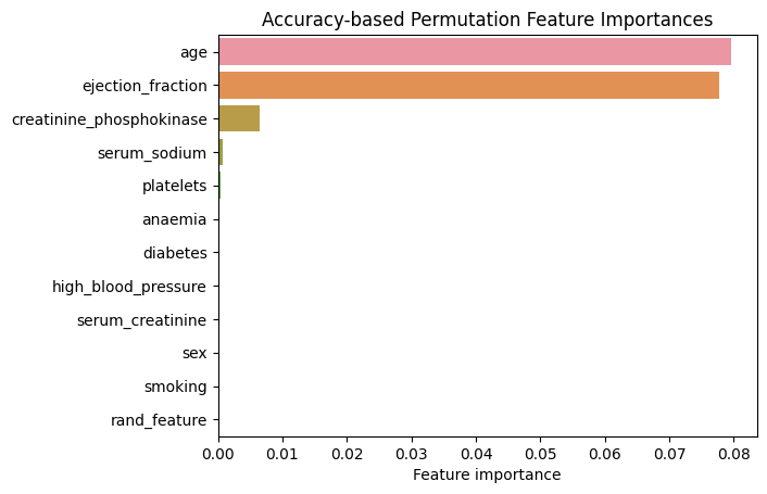
We observe a drastic change in feature importances. There are only three features that appear to have any predictive power: “age”, “ejection_fraction” and “creatinine_phosphokinase”. “serum_creatinine” appears to have completely lost its importance. On the other hand, random feature no longer appears to have any predictive power as should indeed be the case.
References
- Chicco, D., Jurman, G. Machine learning can predict survival of patients with heart failure from serum creatinine and ejection fraction alone. BMC Med Inform Decis Mak 20, 16 (2020). https://doi.org/10.1186/s12911-020-1023-5