Neural Style Transfer

Consider the following image.

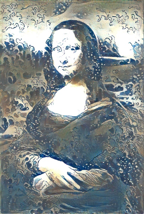
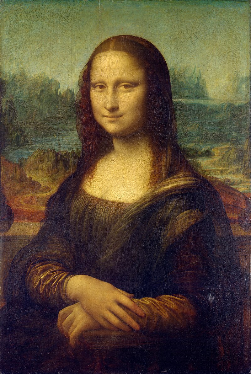
Most of us clearly recognize the famous Mona Lisa by Leonardo da Vinci. However, the style of the image looks quite a bit different from the original painting below.

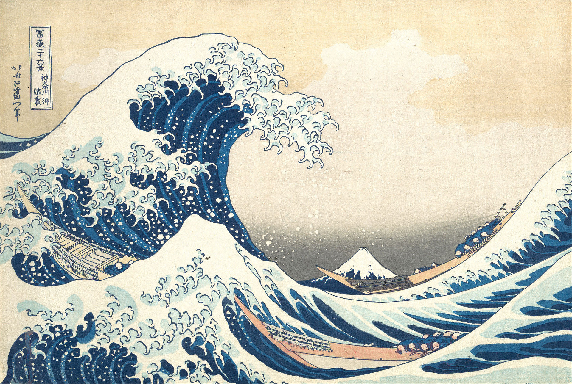
The art connoisseurs among us will recognize that the style is actually borrowed from The Great Wave off Kanagawa by Hokusai.

No, we did not ask a professional artist to create the painting for us which would require quite an effort (it took Leonardo da Vinci four years himself to finish the masterpiece). Instead, such a crossover between art pieces is possible thanks to a class of algorithms known as neural style transfer algorithms.

The problem of merging the contents of one image with the style of another image is not trivial. For us, humans, it is easy to see what constitutes contents of a given image. For example, we would be looking for distinct objects, geometric figures or general scenery. Similarly, when thinking about style of the image, we would pay attention to colors, brush strokes, shades, etc. However, describing all of that programmatically is no easy task. At the end of the day, computers can only see a numeric pixel representation of the image - the same numeric pixel values represent both the contents and the style of the image at the same time. How then do neural style transfer algorithms solve the problem?

In this blog post we will explain how the Neural Algorithm of Artistic Style proposed by Gatys et al. (2016) solves the problem. We will also implement the algorithm using PyTorch library of Python.

Neural Algorithm of Artistic Style

Let us start by properly formulating the problem:

Given content image $c$ and style image $s$, we want to create a new target image $t$ such that $t$ is similar to $c$ in content representation and $t$ is similar to $s$ in style representation.

From the problem definition it becomes clear that solving the problem requires that we be able to extract content representation from image $c$ and style reprensetation from image $s$. This has traditionally been a difficult task. However, recently, there has been a great deal of progress made in our understanding of deep neural network architectures. We now know that deep convolutional neural networks (CNNs), trained on the problem of image classification, do a great job of extracting high-level semantic information from images. Moreover, this information is represented in generic form that generalizes well across various datasets. This insight lies in the heart of the algorithm. According to the authors,

…we use image representations derived from Convolutional Neural Networks optimised for object recognition, which make high level image information explicit. We introduce A Neural Algorithm of Artistic Style that can separate and recombine the image content and style of natural images. The algorithm allows us to produce new images of high perceptual quality that combine the content of an arbitrary photograph with the appearance of numerous well-known artworks.

In the next sections, we explain how we can obtain content and style representations of a given image from a pre-trained CNN.

Content Representation

For any input image $x$ that goes through the network, the feature represenation of the image after application of convolutional layer $l$ can be stored in a feature representation matrix $F^l \in \mathbb{R}^{N_l \times M_l}$, where $N_l$ represents the number of filters used in the layer and $M_l$ is height times width of the feature map. Given the ability of CNNs to represent semantic contents of images, we take this feature representation matrix as the content representation of the image after layer $l$ of the network.

Now using feature representations of images from pre-trained CNNs as their content representations, we define the content loss between the target image $t$ and the content image $c$ at layer $l$ of the neural network, $\mathbb{L}_{content}(t, c, l)$, as follows:

\[\begin{equation} \mathbb{L}\_{content}(t, c, l) = \frac{1}{2} \sum_{i, j}\left(T_{ij}^{l} - C_{ij}^{l}\right)^2, \end{equation}\]

where $T^l$ and $C^l$ are the feature representation matrices of the target and content images after convolutional layer $l$ of the network, respectively. The derivative of the this loss function with respect to the feature representation of the target image at layer $l$ is given by

\[\begin{equation} \frac{\partial \mathbb{L}\_{content}(t, c, l)}{\partial T_{ij}^{l}} = \begin{cases} (T^l - C^l), \text{if } T_{ij}^{l} > 0\\ 0, \text{otherwise} \end{cases} \end{equation}\]

Ability to explicitly estimate the gradient of the content loss with respect to the feature representations of the target image allows us to use gradient descent to minimize this loss, i.e., transform the target image so that its content representation is “closer” to the content representation of the content image at a given layer $l$ of the neural network.

Style Representation

To represent style of a given input image $x$, the authors propose to use Gram matrices. Taking $F^l$ as the feature representation of $x$ at layer $l$ of the network, the corresponding Gram matrix $G^l$ can be estimated in the following way:

\[\begin{equation} G^l = F^l(F^l)^T \end{equation}\]

Taking $G^l$ as style representation of the target image $t$ at layer $l$, denote by $S^l$ style representation of the style image $s$ at layer $l$. We then define style loss at layer $l$, $\mathbb{L}_{l}$, as

\[\begin{equation} \mathbb{L}_{l} = \frac{1}{4N_l^2M_l^2}\sum_{i,j}(G_{i,j}^l - S_{i, j}^l)^2 \end{equation}\]

The total style loss, $\mathbb{L}_{style}$, is the weighted average of losses for individual layers, i.e.,

\[\begin{equation} \mathbb{L}_{style} = \sum_{l=1}^{L}w_l\mathbb{L}_{l}, \end{equation}\]

where $L$ is the total number of layers in the network and $w_l$ is the weight associated with loss for layer $l$. The partial derivatives of $\mathbb{L}_l$ with respect to the feature representation of the target image at layer $l$ are given by

\[\begin{equation} \frac{\partial \mathbb{L_l}}{\partial T_{i, j}^l} = \begin{cases} \frac{1}{N_l^2M_l^2}((T^l)^T(G^l-S^l))_{i, j}, \text{if } T_{i,j}^l > 0\\ 0, \text{otherwise} \end{cases} \end{equation}\]

We can perform gradient descent on the target image $t$ to minimize the mean squared error between the Gram matrices of the target image and the Gram matrices of the style image.

Combined Loss

Having explained how we can obtain content and style representations of images from CNNs, to create a target image $t$ with content representation of content image $c$ and style representation of style image $s$, we minimize, via gradient descent, the following joint loss function:

\[\begin{equation} \mathbb{L}_{combined} = \alpha \mathbb{L}_{content} + \beta \mathbb{L}_{style}, \end{equation}\]

where $\alpha$ and $\beta$ are content loss and style loss weights, respectively.

PyTorch Implementation

In this section, we provide PyTroch implementation of the algorithm. We start by loading the necessary dependencies.

import numpy as np
import pandas as pd
import matplotlib.pyplot as plt
from PIL import Image
import torch
from torch import optim, nn
from torch.nn import functional as F
import torchvision
from torchvision import datasets, transforms
from typing import Dict

To apply the algorithm, we require a convolutional neural network. The authors of the original paper used VGG-19 neural network that was trained to classify images in the well-known ImageNet Large Scale Visual Recognition Challenge. Given the depth and complexity of the model, it would be a daunting task to train it from scratch. Thankfully, torchvision library comes with a pre-trained VGG-19 model and we can load it as follows.

model = torchvision.models.vgg19(pretrained=True)

This network has the following architecture.

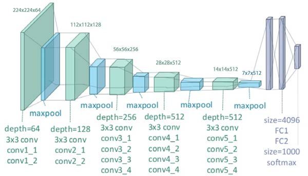
The network can be viewed as consisting of two parts:

• The first part includes five convolutional blocks each followed by max pooling layer. Rectified linear unit (ReLU) activation is applied to outputs of each of the individual convolutional layers. This part is responsible for extracting feature representations of an image.
• The second part consists of three fully connected layers. The first two layers again use the ReLU activation and the final layer uses softmax activation. This part of the VGG-19 network is responsible for image classification.

Given that we are only interested in feature representations of images, we actually do not care about the classification part of the VGG-19 network. Therefore, it can be safely discarded.

feature_model = model.features

Set the parameters of the feature network to be non-trainable as we are not interested in modifying them.

for param in feature_model.parameters():
    param.requires_grad = False

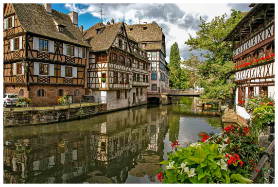
As our content image we choose a nice picture of a town.

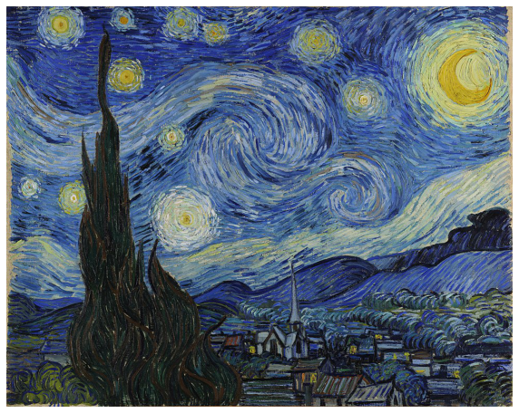
We want our content image to be drawn in the style of The Starry Night by Vincent van Gogh.

Let us define a number of auxiliary functions.

def img_to_tensor(img: Image, width: int=768, height: int=768) -> torch.Tensor:
    """
    Convert input image to torch.Tensor.

    :param img: input image 
    :param width: width of the output image
    :param height: height of the output image
    :return: tensor representation of the input image
    """
    transform = transforms.Compose([transforms.Resize((width, height)),
                                    transforms.ToTensor(),
                                    transforms.Normalize(mean=[0.485, 0.456, 0.406],
                                                         std=[0.229, 0.224, 0.225])])
    tensor = transform(img)
    tensor = tensor.reshape((1, -1, width, height))
    return tensor

def tensor_to_array(tensor: torch.Tensor) -> np.ndarray:
    """
    Convert tensor to numpy.ndarray.

    :param tensor: input tensor
    :return: numpy.ndarray representation of the input tensor
    """
    arr = tensor.clone().detach()
    arr = arr.numpy().squeeze()
    arr = arr.transpose(1,2,0)
    arr = arr * np.array((0.229, 0.224, 0.225)) + np.array((0.485, 0.456, 0.406))
    arr = arr.clip(0, 1)
    return arr

def get_feature_representation(tensor: torch.Tensor, model, layers: Dict[int, str]) -> Dict[int, torch.Tensor]:
    """
    Return a dictionary of feature representations of input image at specified layers of a given model.

    :param tensor: input image as torch.Tensor
    :param model: convolutional neural network model
    :param layers: dictionary of layers for which to return their outputs
    :return: dictionary of feature representations for specified layers
    """
    repr_dict = {}
    x = tensor.clone()
    for name, layer in model._modules.items():
        x = layer(x) 
        if int(name) in layers.keys():
            repr_dict[int(name)] = x
    return repr_dict

def gram_matrix(tensor: torch.Tensor) -> torch.Tensor:
    """
    Estimate Gram matrix.

    :param tensor: input tensor
    :return: gram matrix
    """
    x = tensor.clone()
    x = torch.squeeze(x)
    x = x.reshape(x.shape[0], -1)
    gram_matrix = torch.mm(x, x.T)
    return gram_matrix

def save_image(tensor: torch.Tensor, path: str, name: str) -> None:
    """
    Save torch.Tensor as image.

    :param tensor: input tensor to save as image
    :param path: path to folder where to save the image
    :param name: name of image
    """
    img = Image.fromarray((tensor_to_array(tensor) * 255).astype(np.uint8))
    img.save(path + name)

With all the auxiliary functions defined, we load content and and style images and preprocess them.

content_img = Image.open("city.jpeg")
style_img = Image.open("starry_night.jpeg")

content_tensor = img_to_tensor(content_img, 500, 768)
style_tensor = img_to_tensor(style_img, 500, 768)

We choose feature representations from layer 21 to represent image contents and Gram matrices from layers 0, 5, 10, 19 and 28 to represent image style.

content_layers = {21: 'conv4_2'}
content_repr = get_feature_representation(content_tensor, feature_model, content_layers)

style_layers = {0: 'conv1_1',
                5: 'conv2_1',
                10: 'conv3_1',
                19: 'conv4_1',
                28: 'conv5_1'}
style_repr = get_feature_representation(style_tensor, feature_model, style_layers)
style_gram_matrices = {key: gram_matrix(value) for (key, value) in style_repr.items()}

There is a variety of ways in which a target image can be initialized. For example, a target image can be initialized randomly. Here we will initialize our target image by copying from the content image. Note that we also set requires_grad parameter to True as we want to modify the target image via gradient descent.

target_tensor = content_tensor.clone()
target_tensor.requires_grad = True

We use Adam as the optimizer with a learning rate of 0.005. We use the same loss weights for the style layers. Finally, the weights of content and style losses are set to 1 and 100, respectively.

optimizer = optim.Adam([target_tensor], lr=0.005)
MSE_loss = nn.MSELoss()

style_layer_weights = {0: 0.2,
                       5: 0.2,
                       10: 0.2,
                       19: 0.2,
                       28: 0.2}
alpha = 1
beta = 100

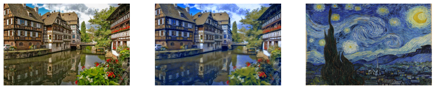
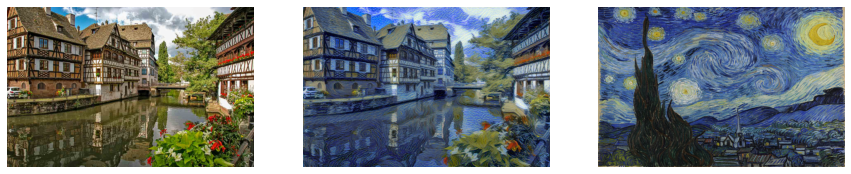
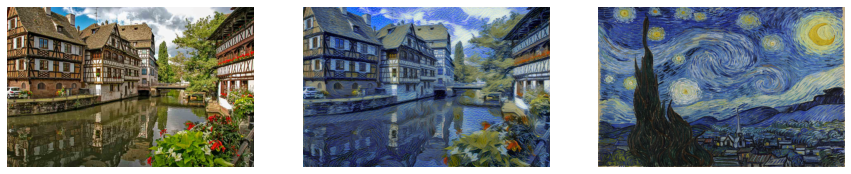
Below we initiate the training process which will be performed over 3,000 epochs. During training we show the progress by printing losses and generated images every 500 epochs.

epochs = 3000
save_every = 500
for e in range(1, epochs + 1):
    loss = 0
    target_content_repr = get_feature_representation(target_tensor, feature_model, content_layers)
    target_style_repr = get_feature_representation(target_tensor, feature_model, style_layers)
    
    feature_model.train()
    optimizer.zero_grad()
    
    content_loss = 0
    for name in content_layers.keys():
        content_loss += MSE_loss(target_content_repr[name], content_repr[name])
    
    style_loss = 0
    for name in style_layers.keys():
        style_loss += MSE_loss(gram_matrix(target_style_repr[name]), style_gram_matrices[name]) * style_layer_weights[name]
        
    loss = alpha * content_loss + beta * style_loss
    
    loss.backward()
    optimizer.step()
    
    if e % save_every == 0:
        print('Epoch {} is over. The loss is {}.'.format(e, loss))
        fig, axs = plt.subplots(1, 3, figsize=(15, 5))
        axs[0].imshow(tensor_to_array(content_tensor))
        axs[0].axis('off')
        axs[1].imshow(tensor_to_array(target_tensor))
        axs[1].axis('off')
        axs[2].imshow(tensor_to_array(style_tensor))
        axs[2].axis('off')
        plt.show();
        
        fig.savefig('img/output/training_progress_{}.png'.format(e))
        save_image(target_tensor, path='img/output/', name='target_img_{}.jpeg'.format(e))

Epoch 500 is over. The loss is 2184042496.0.

Epoch 1000 is over. The loss is 824818048.0.

Epoch 1500 is over. The loss is 457992288.0.

Epoch 2000 is over. The loss is 287117408.0.

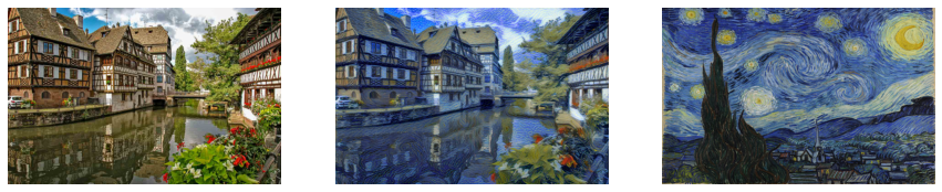
Epoch 2500 is over. The loss is 188992512.0.

Epoch 3000 is over. The loss is 127737632.0.

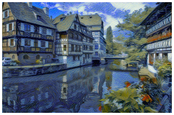
With the training process over, we plot the final image.

fig = plt.figure(figsize=(10, 15))
plt.axis('off')
plt.imshow(tensor_to_array(target_tensor));

Conclusions

The problem of blending contents of a given image with style of another image has traditianlly been very difficult due to inability to extract semantic contents of a given image. This all has changed with the proliferation of deep convolutional neural networks that are getting better and better at problems of image recognition and with that at learning good semantic content representations of images. The Neural Algorithm of Artistic Style is one example from a class of neural style transfer algorithms that utilizes deep CNNs to solve this complex problem.

References

L. A. Gatys, A. S. Ecker, and M. Bethge, “Image style transfer using convolutional neural networks,” in Proceedings of the IEEE Conference on Computer Vision and Pattern Recognition, 2016, pp. 2414–2423.