Local Interpretable Model-Agnostic Explanations
Estimating permutation feature importances and plotting relationships between explanatory variables and model outputs by means of partial dependence plots are important steps in increasing trust in a developed model but they are not enough to really understand how a complex algorithm operates. For model users, decision makers and regulators, it is essential to also understand model outputs to make business decisions while ensuring that the model operates fairly and does not unintentionally discriminate against certain subpopulations. Two popular but different approaches to addressing this “trust” issue are Shapley values, which we will investigate in the following post, and Local Interpretable Model-Agnostic Explanations (LIME).
LIME was introduced in “‘Why Should I Trust You?’ Explaining the Predictions of Any Classifier” by Ribeiro et al. (2016). The key insight of this paper is that prediction of any classifier, regardless of its complexity, at a given point in feature space can be approximated by interpretable models at least in the viscinity of this point. According to the paper, LIME is “…a novel explanation technique that explains the predictions of any classifier in an interpretable and faithful manner, by learning an interpretable model locally around the prediction.” Mathematically, the problem that LIME solves can be expressed as follows:
\[\begin{equation} \xi(x) = \text{argmin}_{g \in G} \mathbb{L}(f, g, \pi_x) + \Omega(g), \end{equation}\]where
- $x\in \mathbb{R}^d$: point in feature space;
- $f: \mathbb{R}^d\rightarrow \mathbb{R}$: classifier whose output needs to be explained at point $x$;
- $\xi(x)$: explanation of $f(x)$;
- $G$: class of interpretable models;
- $\Omega(g)$: measure of complexity of explainer $g$;
- $\pi_x(z)$: measure of proximity of $z$ to $x$;
- $\mathbb{L}(f, g, \pi_x)$: measure of how unfaithful $g$ is in approximating $f$ in the locality of $x$ as defined by $\pi_x$.
The mathematical description of the problem is very general and is open to many interpretations and implementations. For example, the class of interpretable models $G$ may include linear models, like linear regression, tree-based methods, like regression trees, or any other family of models that a user believes is interpretable enough for the task at hand. Similarly, the set of proximity measures $\pi_x$ that can be used is uncountably infinite. All of these choices will affect the way $f(x)$ is explained and will not necessarily agree on the most important features and even on the effects of different features on $f(x)$. Since the purpose of this post is to get a general idea about how LIME works and not to develop a general implementation that would suit different use cases, we will create an implementation with the Ridge regression as the only explainer model. Similarly, we will make a fixed choice with regards to the proximity measure $\pi_x$. The outline of our implementation of LIME algorithm is provided below.
LIME algorithm
Suppose we need to explain $f(x)$, where $f: \mathbb{R}^d \rightarrow \mathbb{R}$ is some complex classifier and $x\in \mathbb{R}^d$. Explanation of $f(x)$ can be obtained via the following steps:
- Perturb $x$ $N$ times to obtain perturbed observations $X’$:
- continuous features: sample from a standard normal distribution and then transform by scaling by the standard deviation of the feature and then by re-centering using the value of the feature at $x$;
- categorical features: sample from the distribution of the feature and convert to a binary variable: 1 if the sampled value is equal to the value of the feature at $x$ and 0 otherwise.
In practice, the shape of $X’$ will be (N + 1, n_features) as the first element of $X’$ will be the transformed version of $x$, $x’$, with categorical features to which binary encoding has been applied;
- Standardize $X’$ and estimate a vector of Euclidean distances, $d$, between $x’$ and observations in $X’$;
-
Convert $d$ to a vector of weights, $w$, via the following kernel function:
\[\begin{equation*} w = \sqrt{e^{\frac{-(d^2)}{k^2}}}, \end{equation*}\]where $k$ is the kernel width. By default, Python implementation of LIME sets $k=\sqrt{\text{n_features}}\times 0.75$.
- Use $f$ to output probabilities of positive class, $p$, on a version of $X’$ from step 1 prior to categorical variables being transformed to a binary variable;
-
Transform $p$ to log odds as follows:
\[\begin{equation*} \text{log odds} = \ln{\frac{p}{1 - p}}; \end{equation*}\] - Use Ridge regression as the explainer model, $g$, and train it on $X’$ to predict log odds from the previous step. Verify that the resulting goodness of fit, as measured by the coefficient of determination, is acceptable;
- Explain $f(x)$ by investigating the predicted log odds from the explainer model, $g(x’)$. The effect of any given feature is then equal to the product of the feature value and the corresponding estimated coefficient of the Ridge regression.
In the next section, we will provide Python implementation of this algorithm.
Python Implementation
Load the required libraries.
import numpy as np
np.random.seed(4)
import pandas as pd
import matplotlib.pyplot as plt
import seaborn as sns

from sklearn.ensemble import RandomForestClassifier
from sklearn.metrics import pairwise_distances
from sklearn.base import BaseEstimator
from sklearn.linear_model import Ridge
from sklearn.preprocessing import StandardScaler
from sklearn.model_selection import train_test_split
from sklearn.feature_selection import SequentialFeatureSelector
from sklearn.utils.validation import check_is_fitted
from sklearn.exceptions import NotFittedError
from sklearn.metrics import roc_auc_score
from sklearn.model_selection import KFold

from lime.lime_tabular import LimeTabularExplainer

from typing import List, Union, Tuple, Optional, Dict, Any
import warnings
warnings.filterwarnings("ignore")
Define p_to_log_odds and log_odds_to_p inverse functions. As their names imply, these functions are used to transform probabilities to log odds and back, respectively.
def p_to_log_odds(p: np.ndarray) -> np.ndarray:
    """
    Transform probabilities to log odds.

    :param p: probabilities
    :return: log odds
    """
    return np.log(p / (1 - p))


def log_odds_to_p(log_odds: np.ndarray) -> np.ndarray:
    """
    Transform log odds to probabilities.

    :param log_odds: log odds
    :return: probabilities
    """
    return 1 / (1 + np.exp(-log_odds))
Below we define LIMExplainer class with the key method - explain_obs.
class LIMExplainer:
    def __init__(self,
                 estimator: BaseEstimator,
                 X: pd.DataFrame,
                 cat_features: List[str]):
        """
        :param estimator: classifier that has been fit to data and whose explanations need to be explained
        :param X: features that have been used to fit `estimator`
        :param cat_features: list of categorical features in `X`. If there are no categorical features,
            provide an empty list
        """
        self._check_estimator(estimator)
        self._estimator = estimator

        self._cat_features = cat_features
        self._cat_features_ids = [i for i, col in enumerate(X.columns) if col in cat_features]
        self._n_cat_features = len(cat_features)
        self._num_features = [col for col in X.columns if col not in cat_features]
        self._num_features_ids = [i for i, col in enumerate(X.columns) if col in self._num_features]
        self._n_num_features = len(self._num_features)
        self._features = list(X.columns)

        if X.isna().any().any():
            raise ValueError("There are missing values in `X`.")
        self._X = X.copy()

        if self._n_num_features > 0:
            self._stds = X[self._num_features].std()

        if self._n_cat_features > 0:
            self._cat_features_dist = {cat_feature: self._X[cat_feature].value_counts() for cat_feature in self._cat_features}


    @staticmethod
    def _check_estimator(estimator: BaseEstimator) -> None:
        """
        Check `estimator`:
        - is instance of `BaseEstimator` class of sklearn;
        - has `predict_proba` method;
        - has been fit to data

        :param estimator: classifier to check
        """
        if not isinstance(estimator, BaseEstimator):
            raise TypeError("`estimator` should be an instance of sklearn `BaseEstimator` class.")

        if "predict_proba" not in dir(estimator):
            raise RuntimeError("There is no `predict_proba` method.")

        try:
            check_is_fitted(estimator)
        except NotFittedError:
            print("The estimator has not been fit to data. Please, fit the estimator to data first.")


    def explain_obs(self,
                    obs: pd.Series,
                    n_features: Optional[Union[int, float, str]]=None,
                    N: Optional[int]=None,
                    dir_feature_selection: str="forward",
                    kernel_width: Optional[float]=None,
                    random_seed: Optional[int]=None):
        """
        Explain observation.

        :param obs: observation to explain which is a pandas Series of features
        :param n_features: number of features to choose for explanation
            - if integer, the number of features;
            - if float between 0 and 1, the fraction of features;
            - if str, can only take a value of `all` in which case all the features will be used
        :param N: number of times to perturb `obs`
        :param dir_feature_selection: if 'forward', perform forward selection, if 'backward' - backward selection
        :param kernel_width: kernel width
        :param random_seed: random seed for reproducibility
        :return: an instance of `Explanation` class
        """
        if len(obs) != len(self._features):
            raise RuntimeError(f"Shape of `obs` should be ({len(self._features)},).")

        if n_features is None:
            n_features = "auto"
        elif isinstance(n_features, str):
            if n_features != "all":
                raise ValueError("if string, `n_features` can only be equal to 'all'.")

        if not N:
            N = max(1000, 30 * len(obs))
        else:
            if not isinstance(N, int) or N < 1:
                raise ValueError("`N` should be a positive integer.")

        if random_seed:
            np.random.seed(random_seed)

        perturbed_sample, perturbed_sample_encoded = self._perturb_obs(obs, N)

        scaled_sample = StandardScaler().fit_transform(perturbed_sample_encoded)
        distances = pairwise_distances(scaled_sample[1:], scaled_sample[0].reshape(1, -1)).flatten()

        weights = self._convert_distances_to_weights(distances, kernel_width)

        preds = self._estimator.predict_proba(perturbed_sample)[:, 1]
        preds = p_to_log_odds(preds)

        if n_features != "all":
            selected_features = self._select_features(X=perturbed_sample_encoded,
                                                      y=preds,
                                                      n_features=n_features,
                                                      direction=dir_feature_selection)
        else:
            selected_features = self._features

        X = perturbed_sample_encoded[selected_features].values

        self.explainer = Ridge()
        self.explainer.fit(X[1:], preds[1:], weights)

        explainer_score = self.explainer.score(X[1:], preds[1:], weights)

        local_prediction = self.explainer.predict(X[0].reshape(1, -1))
        local_prediction = log_odds_to_p(local_prediction)

        return Explanation(obs=obs,
                           features=selected_features,
                           intercept=self.explainer.intercept_,
                           coef=self.explainer.coef_,
                           r2=explainer_score,
                           local_pred=local_prediction)


    def _perturb_obs(self,
                     obs: pd.Series,
                     N: int) -> Tuple[pd.DataFrame, pd.DataFrame]:
        """
        Perturb `obs` and return a tuple of
        - perturbed sample with shape (N + 1, n_features)
        - perturbed sample with binary encoding of categorical features with shape (N + 1, n_features)

        :param obs: observation to perturb
        :param N: number of times to perturn `obs`
        :return: perturbed sample and perturbed sample with categorical features encoded
        """
        N = N + 1 # add one as the first observation will be `obs` itself

        if self._n_num_features > 0:
            std_norm_sample = np.random.normal(0, 1, (N, self._n_num_features))
            perturbed_num_features = std_norm_sample * self._stds.values + obs[self._num_features_ids].values
            perturbed_num_features = pd.DataFrame(perturbed_num_features, columns=self._num_features)
            perturbed_num_features.iloc[0, :] = obs[self._num_features_ids]
        else:
            perturbed_num_features = pd.DataFrame()

        perturbed_cat_features = pd.DataFrame()
        perturbed_cat_features_encoded = pd.DataFrame()
        if self._n_cat_features > 0:
            for cat_feature in self._cat_features:
                dist = self._cat_features_dist[cat_feature]
                vals = dist.index
                p = dist / dist.sum()
                perturbed_cat_features[cat_feature] = np.random.choice(vals, size=N, p=p)
            perturbed_cat_features.iloc[0, :] = obs[self._cat_features_ids]
            perturbed_cat_features_encoded = (perturbed_cat_features==obs[self._cat_features_ids]).astype(int)

        perturbed_sample = pd.concat([perturbed_num_features, perturbed_cat_features], axis=1)
        perturbed_sample = perturbed_sample[self._features]

        perturbed_sample_encoded = pd.concat([perturbed_num_features, perturbed_cat_features_encoded], axis=1)
        perturbed_sample_encoded = perturbed_sample_encoded[self._features]

        return perturbed_sample, perturbed_sample_encoded


    def _convert_distances_to_weights(self,
                                      distances: np.ndarray,
                                      kernel_width: Optional[float]=None) -> np.ndarray:
        """
        Convert distances to weights using kernel function.

        :param: distances: distances
        :param kernel_width: kernel width
        :return: weights
        """
        if (distances < 0).any():
            raise ValueError("`distances` cannot contain negative values.")

        if kernel_width is None:
            kernel_width = np.sqrt(len(self._features)) * 0.75
        elif kernel_width <= 0:
            raise ValueError("`kernel_width` should be a positive number.")

        weights = np.sqrt(np.exp(-(distances)**2 / kernel_width**2))

        return weights / weights.sum()


    def _select_features(self,
                         X: pd.DataFrame,
                         y: np.ndarray,
                         n_features: Union[int, float, str],
                         direction: str="forward") -> List[str]:
        """
        Select most predictive features.

        :param X: training observations with shape (n_observations, n_features)
        :param y: labels
        :param n_features: number of features to choose for explanation
            - if integer, the number of features;
            - if float between 0 and 1, the fraction of features
        :param direction: if 'forward', perform forward selection, if 'backward' - backward selection
        :return: names of the chosen features
        """
        feature_selector = SequentialFeatureSelector(estimator=Ridge(),
                                                     n_features_to_select=n_features,
                                                     direction=direction)

        feature_selector.fit(X, y)
        return feature_selector.get_feature_names_out()
explain_obs method of LIMExplainer class outputs an instance of Explanation class that we define below.
class Explanation:
    def __init__(self,
                 obs: pd.Series,
                 features: List[str],
                 intercept: float,
                 coef: np.ndarray,
                 r2: float,
                 local_pred: float):
        """
        :param obs: observation
        :param features: features
        :param intercept: intercept of the fitted Ridge regression
        :param coef: coefficients of the fitted Ridge regression
        :param r2: coefficient of determination of the fitted Ridge regression
        :param local_pred: probability of positive class obtained from the fitted Ridge regression at `obs`
        """
        self._obs = obs
        self._features = features
        self._intercept = intercept
        self._coef = coef
        self._feature_effects = pd.DataFrame({"Feature": [f"{pair[0]}={pair[1]}" for pair in zip(features, obs.values)],
                                              "Effect on positive class": obs.values * coef}
                                            ).sort_values(by="Effect on positive class", ascending=False, key=abs)
        self._r2 = r2
        self._local_pred = local_pred

    @property
    def obs(self) -> pd.Series:
        return self._obs

    @property
    def feature_effects(self) -> pd.DataFrame:
        return self._feature_effects

    @property
    def features(self) -> List[str]:
        return self._features

    @property
    def intercept(self) -> float:
        return self._intercept

    @property
    def coef(self) -> np.ndarray:
        return self._coef

    @property
    def r2(self) -> float:
        return self._r2

    @property
    def local_pred(self) -> float:
        return self._local_pred


    def plot(self, figsize: Tuple[int, int]=(10, 5)) -> plt.Figure:
        """
        Return plot of feature effects.

        :param figsize: figure size
        :return: plot of feature effects
        """
        fig = plt.figure(figsize=figsize)
        sns.barplot(self.feature_effects, x="Effect on positive class", y="Feature")
        plt.close()
        return fig
Now that we have implemented the algorithm, we can test its implementation on real data. We continue using the same heart failure clinical records dataset that we used in the preceding two posts on model explainability: Partial Dependence Plots and Permutation Feature Importance. The dataset can be downloaded from UC Irvine Machine Learning Repository.
df = pd.read_csv("data/heart_failure_clinical_records_dataset.csv")
df.columns = [col.lower() for col in df.columns]
print(f"Dataset shape: {df.shape}")
df.head()
Dataset shape: (299, 13)
| age | anaemia | creatinine_phosphokinase | diabetes | ejection_fraction | high_blood_pressure | platelets | serum_creatinine | serum_sodium | sex | smoking | time | death_event | |
|---|---|---|---|---|---|---|---|---|---|---|---|---|---|
| 0 | 75.0 | 0 | 582 | 0 | 20 | 1 | 265000.00 | 1.9 | 130 | 1 | 0 | 4 | 1 |
| 1 | 55.0 | 0 | 7861 | 0 | 38 | 0 | 263358.03 | 1.1 | 136 | 1 | 0 | 6 | 1 |
| 2 | 65.0 | 0 | 146 | 0 | 20 | 0 | 162000.00 | 1.3 | 129 | 1 | 1 | 7 | 1 |
| 3 | 50.0 | 1 | 111 | 0 | 20 | 0 | 210000.00 | 1.9 | 137 | 1 | 0 | 7 | 1 |
| 4 | 65.0 | 1 | 160 | 1 | 20 | 0 | 327000.00 | 2.7 | 116 | 0 | 0 | 8 | 1 |
Summary statistics of the dataset is provided below.
def describe_df(df: pd.DataFrame) -> pd.DataFrame:
    """
    Describe pandas dataframe.

    :param df: input dataframe
    :return: description of the dataset
    """
    col_types = df.dtypes
    col_types.name = "dtype"

    n_missing = df.isna().astype(int).sum(axis=0)
    n_missing.name = "n_missing"

    pct_missing = n_missing / len(df)
    pct_missing.name = "pct_missing"

    n_unique = df.nunique()
    n_unique.name = "n_unique"

    skewness = df.skew()
    skewness.name = "skewness"

    kurtosis = df.kurt()
    kurtosis.name = "kurtosis"

    return pd.concat([col_types, n_missing, pct_missing, n_unique, df.describe().T, skewness, kurtosis],
                     axis=1)

describe_df(df)
| dtype | n_missing | pct_missing | n_unique | count | mean | std | min | 25% | 50% | 75% | max | skewness | kurtosis | |
|---|---|---|---|---|---|---|---|---|---|---|---|---|---|---|
| age | float64 | 0 | 0.0 | 47 | 299.0 | 60.833893 | 11.894809 | 40.0 | 51.0 | 60.0 | 70.0 | 95.0 | 0.423062 | -0.184871 |
| anaemia | int64 | 0 | 0.0 | 2 | 299.0 | 0.431438 | 0.496107 | 0.0 | 0.0 | 0.0 | 1.0 | 1.0 | 0.278261 | -1.935563 |
| creatinine_phosphokinase | int64 | 0 | 0.0 | 208 | 299.0 | 581.839465 | 970.287881 | 23.0 | 116.5 | 250.0 | 582.0 | 7861.0 | 4.463110 | 25.149046 |
| diabetes | int64 | 0 | 0.0 | 2 | 299.0 | 0.418060 | 0.494067 | 0.0 | 0.0 | 0.0 | 1.0 | 1.0 | 0.333929 | -1.901254 |
| ejection_fraction | int64 | 0 | 0.0 | 17 | 299.0 | 38.083612 | 11.834841 | 14.0 | 30.0 | 38.0 | 45.0 | 80.0 | 0.555383 | 0.041409 |
| high_blood_pressure | int64 | 0 | 0.0 | 2 | 299.0 | 0.351171 | 0.478136 | 0.0 | 0.0 | 0.0 | 1.0 | 1.0 | 0.626732 | -1.618076 |
| platelets | float64 | 0 | 0.0 | 176 | 299.0 | 263358.029264 | 97804.236869 | 25100.0 | 212500.0 | 262000.0 | 303500.0 | 850000.0 | 1.462321 | 6.209255 |
| serum_creatinine | float64 | 0 | 0.0 | 40 | 299.0 | 1.393880 | 1.034510 | 0.5 | 0.9 | 1.1 | 1.4 | 9.4 | 4.455996 | 25.828239 |
| serum_sodium | int64 | 0 | 0.0 | 27 | 299.0 | 136.625418 | 4.412477 | 113.0 | 134.0 | 137.0 | 140.0 | 148.0 | -1.048136 | 4.119712 |
| sex | int64 | 0 | 0.0 | 2 | 299.0 | 0.648829 | 0.478136 | 0.0 | 0.0 | 1.0 | 1.0 | 1.0 | -0.626732 | -1.618076 |
| smoking | int64 | 0 | 0.0 | 2 | 299.0 | 0.321070 | 0.467670 | 0.0 | 0.0 | 0.0 | 1.0 | 1.0 | 0.770349 | -1.416080 |
| time | int64 | 0 | 0.0 | 148 | 299.0 | 130.260870 | 77.614208 | 4.0 | 73.0 | 115.0 | 203.0 | 285.0 | 0.127803 | -1.212048 |
| death_event | int64 | 0 | 0.0 | 2 | 299.0 | 0.321070 | 0.467670 | 0.0 | 0.0 | 0.0 | 1.0 | 1.0 | 0.770349 | -1.416080 |
We will make use of stratified sampling to split the dataset into training and test sets. We will keep the proportion of test set observations equal to 0.2.
TARGET = "death_event"
FEATURES = [col for col in df.columns if col not in [TARGET, "time"]]
CAT_FEATURES = ["anaemia", "diabetes", "high_blood_pressure", "sex", "smoking"]
X = df[FEATURES]
y = df[TARGET]
X_train, X_test, y_train, y_test = train_test_split(X, y, test_size=0.2, random_state=4, stratify=y)
Next we fit a random forest classifier to the training dataset and check model fit using area under receiver operating characteristic (AUROC).
estimator = RandomForestClassifier(n_estimators=28,
                                   max_depth=4,
                                   min_samples_split=0.16,
                                   min_samples_leaf=0.024,
                                   max_features='sqrt')
estimator.fit(X_train, y_train)
train_auroc = roc_auc_score(y_train, estimator.predict_proba(X_train)[:, 1])
test_auroc = roc_auc_score(y_test, estimator.predict_proba(X_test)[:, 1])
print(f"Train AUROC: {round(train_auroc, 4)}")
print(f"Test AUROC: {round(test_auroc, 4)}")
Train AUROC: 0.8846
Test AUROC: 0.7792
Judging by the AUROC achieved on both the training and test sets, it appears that the random forest classifier possesses discriminatory power in differentiating between positive (death) and negative (survival) classes.
We proceed by investigating feature importances learned by the classifier on the training sample. For that purpose, RandomForestClassifier class of sklearn has feature_importances_ attribute.
feature_importances_tree = pd.DataFrame({"features": FEATURES,
                                         "importance": estimator.feature_importances_}).sort_values(by="importance", ascending=False)
sns.barplot(feature_importances_tree, y="features", x="importance");
Figure 1. Feature Importances
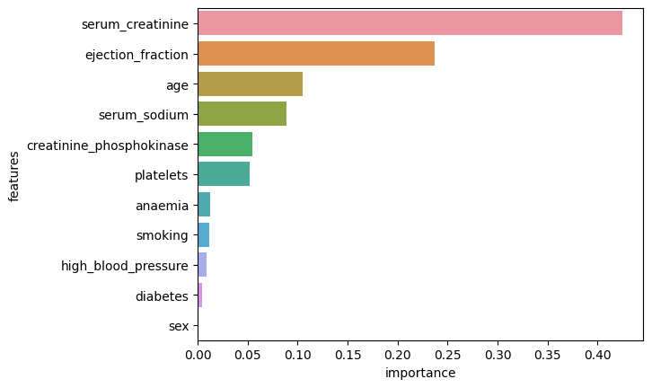
The two most important features are “serum_creatinine” and “ejection_fraction” which is in agreement with the observations by Chicco and Jurman (2020) who analysed the same dataset.
Let us now obtain probabilities of positive class on the test set from the classifier.
p_pos_class_test = estimator.predict_proba(X_test)[:, 1]
y_pred_test = pd.DataFrame({"true_label": y_test,
                            "probability_pos_class": p_pos_class_test,
                            "abs_diff": np.abs(y_test - p_pos_class_test)}).sort_values(by="abs_diff", ascending=False)
y_pred_test.index.name = "patient_ID"
The table below shows the top five observations in the test set where the classifier makes the most “incorrect” predictions.
y_pred_test.head(5)
| true_label | probability_pos_class | abs_diff | |
|---|---|---|---|
| patient_ID | |||
| 22 | 1 | 0.143059 | 0.856941 |
| 42 | 1 | 0.182561 | 0.817439 |
| 164 | 1 | 0.282386 | 0.717614 |
| 190 | 0 | 0.666923 | 0.666923 |
| 105 | 1 | 0.347894 | 0.652106 |
As such, the random forest classifier assigned a probability of death of only 14.3% to the patient with ID=22. However, the true label associated with this patient is 1, i.e., the patient ended up dying. To understand why the algorithm made such a big “error”, let us use the LIMExplainer class that we defined.
explainer = LIMExplainer(estimator=estimator,
                         X=X_train,
                         cat_features=CAT_FEATURES)
explanation = explainer.explain_obs(X_test.loc[22, :], n_features="all", random_seed=4)
Let us first investigate the goodness of fit of the Ridge regression and the local prediction.
print(f"Coefficient of determination: {explanation.r2}")
print(f"Local prediction: {explanation.local_pred}")
Coefficient of determination: 0.5501182037760741
Local prediction: [0.31381603]
The obtained coefficient of determination is equal to 0.55. This means that about 55% of the variation in the log odds from the random forest classifier is explained by the Ridge regression model.
The local prediction from the Ridge regression is equal to 0.31. Therefore, the explainer model agrees with the random forest classifier on the most probable class for the patient.
To see why the local prediction is like that, we plot the effects of different feature values on the prediction below.
explanation.plot()
Figure 2. Explanation. LIMExplainer
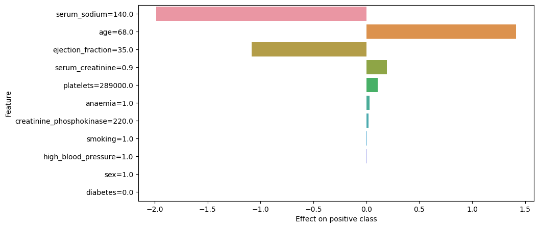
As becomes clear from the above plot, the main reasons for why the explainer model sees this observation as being more likely to belong to class 0 are the value of 140 for “serum_sodium” and the value of 35 for “ejection_fraction” features. As a reminder, these features are the fourth and the second most important features to the random forest classifier, respectively.
Since these variables can only take positive values, it implies that the corresponding coefficients in the Ridge regression for these variables are negative. Let us check the coefficients next to confirm if this is indeed the case.
pd.DataFrame({"feature": explanation.features,
              "coefficient": explanation.coef})
| feature | coefficient | |
|---|---|---|
| 0 | age | 2.080070e-02 |
| 1 | anaemia | 2.927698e-02 |
| 2 | creatinine_phosphokinase | 8.888221e-05 |
| 3 | diabetes | -6.093930e-03 |
| 4 | ejection_fraction | -3.095574e-02 |
| 5 | high_blood_pressure | 3.892387e-03 |
| 6 | platelets | 3.781060e-07 |
| 7 | serum_creatinine | 2.179444e-01 |
| 8 | serum_sodium | -1.417517e-02 |
| 9 | sex | 3.462804e-04 |
| 10 | smoking | 7.299218e-03 |
Indeed, the coefficient for “serum_sodium” feature is -0.01418 and the coefficient for “ejection_fraction” feature is -0.03096.
Negative coefficients imply that there are inverse relationships between these variables and predicted probabilities of positive class from the random forest classifier. To confirm this, we plot partial dependence plots for these features below.
def partial_dependence_1d(estimator: BaseEstimator,
                          X: pd.DataFrame,
                          feature: Union[List[str], str]) -> pd.Series:
    """
    Partial dependence for `feature`.

    :param estimator: estimator that has been fit to data
    :param X: dataframe of features with shape (N_samples, N_features)
    :param feature: feature for which partial dependence is estimated
    :return: estimated partial dependence
    """
    LIMExplainer._check_estimator(estimator)
    if isinstance(feature, list):
        feature = feature[0]
    assert feature in X.columns, f"`{feature}` column could not be found in the dataframe."

    X = X.copy()
    unique_vals = np.sort(X[feature].unique())
    res = pd.Series(np.zeros_like(unique_vals), index=unique_vals, name=feature)
    for i, val in enumerate(unique_vals):
        X[feature] = val
        preds = estimator.predict_proba(X.values)[:, 1]
        res.iloc[i] = np.mean(preds, axis=0)
    return res


def partial_dependence_plot_1d(estimator: BaseEstimator,
                               X: pd.DataFrame,
                               feature: Union[str, List[str]],
                               figsize: Tuple=(10, 5)) -> plt.Figure:
    """
    Return partial dependence plot for a single target feature.

    :param estimator: estimator that has been fit to data
    :param X: dataframe of features with shape (N_samples, N_features)
    :param feature: target feature
    :param figsize: size of plot
    :return: partial dependence plot
    """
    if isinstance(feature, list):
        feature = feature[0]
    pd = partial_dependence_1d(estimator, X, feature)
    fig = plt.figure(figsize=figsize)
    plt.plot(pd)
    plt.ylabel("Partial Dependence")
    plt.xlabel(f"{pd.name}")
    if len(pd) < 10:
        plt.xticks(pd.index)
    plt.grid()
    plt.close()
    return fig
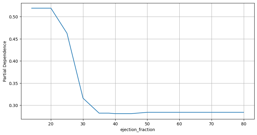
partial_dependence_plot_1d(estimator, X_train, "ejection_fraction")
Figure 3. Partial Dependence Plot. Ejection Fraction
partial_dependence_plot_1d(estimator, X_train, "serum_sodium")
Figure 4. Partial Dependence Plot. Serum Sodium
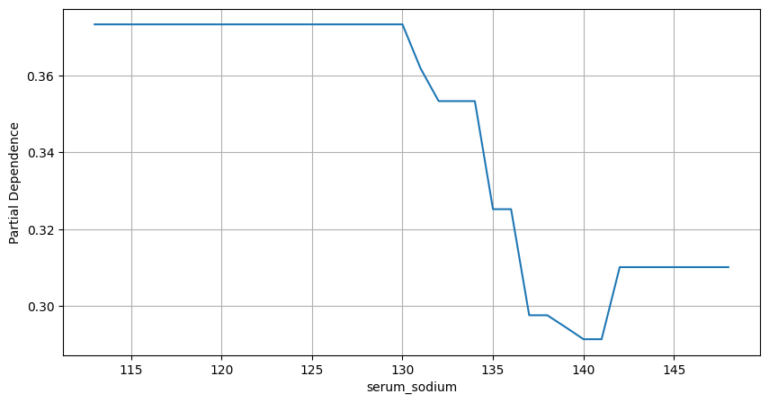
Partial dependence plots confirm that higher values for these variables are associated with lower probabilities of belonging to class 1.
On the other hand, the value of 68 for “age” variable increases the probability of positive class as predicted by the explainer model. This is not surprising as older people are more likely to die following a heart failure event and the average patient age in the sample is 60.8. Thus, the model correctly believes that the patient’s age increases his or hers chances of not surviving.
The values for other variables, like “serum_creatinine”, “platelets”, “anaemia”, “creatinine_phosphokinase”, have the same directional effect as “age” but the corresponding magnitudes are low.
Finally, we will use LIME package to explain the same observation to see if its explanation aligns with what we have seen so far. To that end, we will use explain_instance method of LimeTabularExplainer class.
def predict_fn(X: np.ndarray) -> np.ndarray:
    return estimator.predict_proba(X)

lime_explainer = LimeTabularExplainer(training_data=X_train,
                                      training_labels=y_train,
                                      feature_names=FEATURES,
                                      categorical_names=CAT_FEATURES,
                                      discretize_continuous=False,
                                      random_state=4)

lime_explanation = lime_explainer.explain_instance(data_row=X_test.loc[22, :].values,
                                                   predict_fn=predict_fn,
                                                   num_samples=1000,
                                                   num_features=len(FEATURES))
print(f"Coefficient of determination: {lime_explanation.score}")
print(f"Local prediction: {lime_explanation.local_pred}")
Coefficient of determination: 0.6260917511928257
Local prediction: [0.31870942]
The local prediction of 0.32 is very close to the local prediction of 0.31 that we have obtained from LIMExplainer. However, the coefficient of determination from LimeTabularExplainer of 0.63 is higher.
Below we plot the effects of different features on the predicted probability of positive class.
lime_explanation.show_in_notebook()
Figure 5. Explanation. LimeTabularExplainer
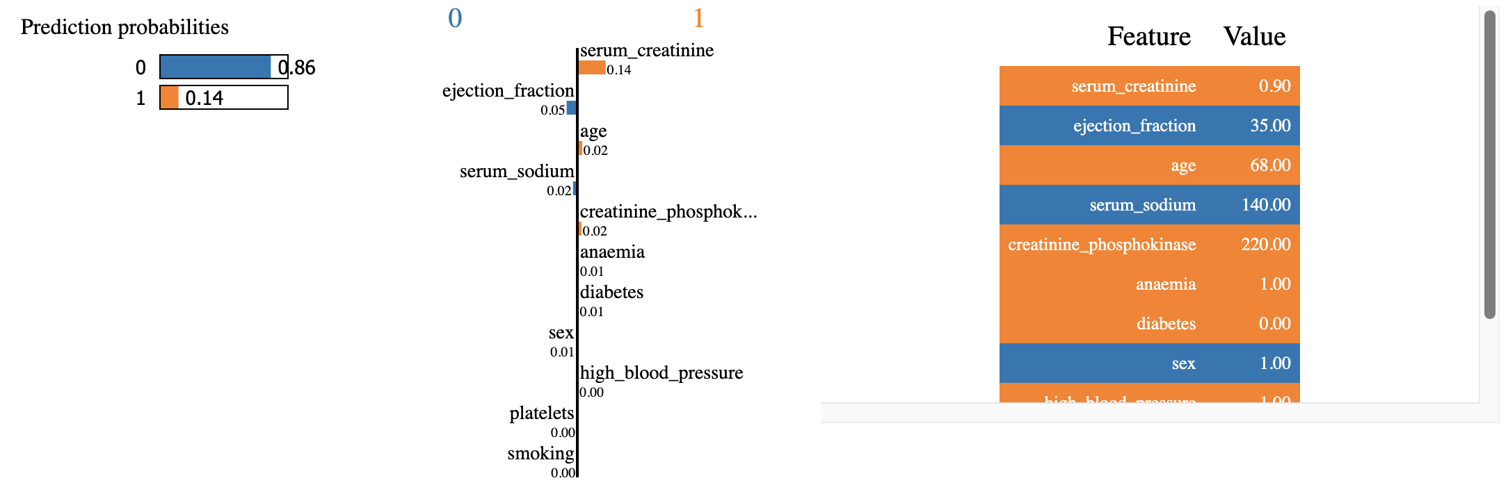
While the two explanations agree on the directional effects of the values of the features, they disagree on the magnitudes of their effects. As such, according to LimeTabularExplainer, the most important support for class 0 prediction is the value of 35 for “ejection_fraction” feature. This is followed by the value of 140 for “serum_sodium”. On the other hand, the value of 0.9 for “serum_creatinine” is deemed to be the most significant evidence in support of class 1 prediction.
References
- Chicco, D., Jurman, G. Machine learning can predict survival of patients with heart failure from serum creatinine and ejection fraction alone. BMC Med Inform Decis Mak 20, 16 (2020). https://doi.org/10.1186/s12911-020-1023-5