Introduction to Kalman Filter

In this post, we cover the theory behind a discrete-time Kalman filter. Kalman filter is an algorithm that allows us to get a more precise information about a state of dynamically developing systems by incorporating information taken from measurements. Of course, both the system and the measurements are subject to distortions caused by uncontrollable noise. The algorithm works by incorporating information from our knowledge of how a given system develops and uncertainty surrounding the measurement devices to get an overall more precise estimate. Ever since its development in the 1960s, the filter has found applications in many domains and is frequently used in control theory applications, time series analysis, navigation, etc.

Mathematical Background

To properly understand how Kalman filtering works, we are going to first cover the necessary mathematical background. This will make subsequent derivations much more transparent. We are following closely the material covered by Simon (2006).

We are sticking to the following notational conventions: upper-case letters stand for matrices, bold lower-case letters represent vectors, and lower-case letters stand for constants and random variables.

Linear Dynamical Systems

Suppose that we have the following discrete-time linear system:

\[\begin{equation} \boldsymbol{x}_{t} = F_{t-1}\boldsymbol{x}_{t-1} + G_{t-1}\boldsymbol{u}_{t-1} + \boldsymbol{w}_{t-1}, \label{eq:linear_system} \end{equation}\]

where $\boldsymbol{u}$ is known input to the system and $G$ is its associated matrix, $F$ is state transition matrix and $\boldsymbol{w_{t-1}} \sim N\left(\boldsymbol{0}, Q_{t-1}\right)$. Let $\bar{\boldsymbol{x_t}}$ and $P_{t}$ denote the expectation and the variance-covariance matrix of the random vector $\boldsymbol{x}_{t}$. We are interested in how the expectation and the variance-covariance matrix propagate through time. Consider the expectation first.

\[\begin{align} \bar{\boldsymbol{x}}_t &= E\left[F_{t-1}\boldsymbol{x}_{t-1} + G_{t-1}\boldsymbol{u}_{t-1} + \boldsymbol{w}_{t-1}\right] \nonumber \\ &= F_{t-1}E[\boldsymbol{x}_{t-1}] + G_{t-1}\boldsymbol{u}_{t-1} \nonumber \\ &= F_{t-1}\bar{\boldsymbol{x}}_{t-1} + G_{t-1}\boldsymbol{u}_{t-1}. \label{eq:mean_propagation} \end{align}\]

Next consider the variance-covariance matrix.

\[\begin{align*} P_t &= E\left[\left(\boldsymbol{x}_t - \bar{\boldsymbol{x}}_t\right)\left(\boldsymbol{x}_t - \bar{\boldsymbol{x}}_t\right)^T\right]\\ &= E\left[\left(F_{t-1}\boldsymbol{x}_{t-1} + \boldsymbol{w}_{t-1} - F_{t-1}\bar{\boldsymbol{x}}_{t-1}\right)\left(F_{t-1}\boldsymbol{x}_{t-1} + \boldsymbol{w}_{t-1} - F_{t-1}\bar{\boldsymbol{x}}_{t-1}\right)^T\right]\\ &= E\left[\left(F_{t-1}\left(\boldsymbol{x}_{t-1} - \bar{\boldsymbol{x}}_{t-1}\right) + \boldsymbol{w}_{t-1}\right)\left(F_{t-1}\left(\boldsymbol{x}_{t-1} - \bar{\boldsymbol{x}}_{t-1}\right) + \boldsymbol{w}_{t-1}\right)^T\right] \\ &= E\left[F_{t-1}\left(\boldsymbol{x}_{t-1} - \bar{\boldsymbol{x}}_{t-1}\right)\left(\boldsymbol{x}_{t-1} - \bar{\boldsymbol{x}}_{t-1}\right)^T F_{t-1}^T \right] + E\left[F_{t-1}\left(\boldsymbol{x}_{t-1} - \bar{\boldsymbol{x}}_{t-1}\right)\boldsymbol{w}_{t-1}^{T}\right] + E\left[\boldsymbol{w}_{t-1} \left(\boldsymbol{x}_{t-1} - \bar{\boldsymbol{x}}_{t-1}\right)^T F_{t-1}^T\right] + E\left[\boldsymbol{w}_{t-1}\boldsymbol{w}_{t-1}^T\right]. \end{align*}\]

Since $\boldsymbol{w_{t-1}}$ is independent of $\boldsymbol{x_{t-1}} - \bar{\boldsymbol{x_{t-1}}}$ and $E\left[\boldsymbol{w_{t-1}}\right] = \boldsymbol{0}$, we have

\[\begin{align} P_t &= F_{t-1}E\left[\left(\boldsymbol{x}_{t-1} - \bar{\boldsymbol{x}}_{t-1}\right)\left(\boldsymbol{x}_{t-1} - \bar{\boldsymbol{x}}_{t-1}\right)^T\right]F_{t-1}^T + Q_{t-1} \nonumber \\ &= F_{t-1}P_{t-1}F_{t-1}^T + Q_{t-1}. \label{eq:variance_propagation} \end{align}\]

Assuming that $F$ and $G$ are deterministic, $\boldsymbol{x}_t$ will be normally distributed. Knowing how the expectation and the variance-covariance matrix of the state evolves through time we can already characterize our state variable $\boldsymbol{x}_t$ at any time $t$ as follows

\[\begin{equation*} \boldsymbol{x}_t \sim N\left(\bar{\boldsymbol{x}}_t, P_t\right). \end{equation*}\]

Example

Let $x_t^{(1)}$ be a random variable that represents the population of some tribe at time $t$ and $x_t^{(2)}$ be a random variable that represents the supply of food at time $t$. Consider the following system:

\[\begin{align*} x_t^{(1)} &= x_{t-1}^{(1)} - 0.4x_{t-1}^{(1)} + 0.2x_{t-1}^{(2)} + w_{t-1}^{(1)}\\ x_t^{(2)} &= x_{t-1}^{(2)} - 0.2x_{t-1}^{(1)} + u + w_{t-1}^{(2)}, \end{align*}\]

where $u$ is constant change in supply of food, e.g. our tribe is engaged in growing crop. We can rewrite the above system in matrix form as follows:

\[\begin{align*} \boldsymbol{x}_t = \left( \begin{matrix} 0.6 & 0.2 \\ -0.2 & 1 \end{matrix} \right) \left( \begin{matrix} x_{t-1}^{(1)} \\ x_{t-1}^{(2)} \end{matrix} \right) + \left( \begin{matrix} 0 \\ u \end{matrix} \right) + \left( \begin{matrix} w_{t-1}^{(1)} \\ w_{t-1}^{(2)} \end{matrix} \right). \end{align*}\]

Suppose we know the initial distribution of the state of the system, i.e.

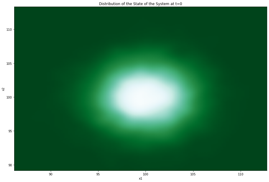
\[\begin{align*} \bar{\boldsymbol{x}}_0 &= \left( \begin{matrix} 100 \\ 100 \end{matrix} \right), \\ P_0 &= \left( \begin{matrix} 10 & 0 \\ 0 & 10 \end{matrix} \right). \end{align*}\]

Below we are plotting a Gaussian blob that represents our knowledge of the state of the system at time 0.

import numpy as np
import matplotlib.pyplot as plt
from scipy.stats import kde

mean_0 = [100, 100]

P_0 = [[10, 0], [0, 10]]

np.random.seed(4)
data = np.random.multivariate_normal(mean_0, P_0, 10000)
nbins = 100
x = data[:, 0]
y = data[:, 1]
k = kde.gaussian_kde(data.T)
xi, yi = np.mgrid[x.min():x.max():nbins*1j, y.min():y.max():nbins*1j]
zi = k(np.vstack([xi.flatten(), yi.flatten()]))

fig = plt.figure(figsize=(15, 10))
ax = fig.add_subplot(1,1,1)
ax.pcolormesh(xi, yi, zi.reshape(xi.shape), shading='gouraud', cmap=plt.cm.BuGn_r)
plt.xlabel('x1')
plt.ylabel('x2')
plt.title('Distribution of the State of the System at t=0')

Since we know how the mean and the variance-covariance matrix of the system propagate through time, we can get an idea of the distribution of the system at some future time assuming that the system develops in accordance with Equation $\left(\ref{eq:linear_system}\right)$. For example, let us see what the distribution of the state looks like at time $t=10$. Assume that $u=5$ and

\[\begin{align*} \boldsymbol{w}_t &\sim N \left(\boldsymbol{0}, Q\right) \\ &\sim N\left( \left( \begin{matrix} 0 \\ 0 \end{matrix} \right), \left( \begin{matrix} 1 & 0 \\ 0 & 1 \end{matrix} \right) \right). \end{align*}\]

Since our state transition matrix $F$ is constant over time and $G$ is the identity matrix, the change in the expectation of the state of the system can be expressed as

\[\begin{align*} \bar{\boldsymbol{x}}_t &= F\bar{\boldsymbol{x}}_{t-1} + \boldsymbol{u} \\ &= \left( \begin{matrix} 0.6 & 0.2 \\ -0.2 & 1 \end{matrix} \right) \left( \begin{matrix} \bar{x}_{t-1}^{(1)} \\ \bar{x}_{t-1}^{(2)} \end{matrix} \right) + \left( \begin{matrix} 0 \\ 5 \end{matrix} \right). \end{align*}\]

The change in the variance-covariance matrix of the state of the system changes according to

\[\begin{align*} P_t &= FP_{t-1}F^T + Q \\ &= \left( \begin{matrix} 0.6 & 0.2 \\ -0.2 & 1 \end{matrix} \right) P_{t-1} \left( \begin{matrix} 0.6 & -0.2 \\ 0.2 & 1 \end{matrix} \right) + \left( \begin{matrix} 1 & 0 \\ 0 & 1 \end{matrix} \right). \end{align*}\]

Let us propagate the expectation and the variance-covariance matrix of the system to time $t=10$ according to the above equations.

t = 10
F = np.array([[0.6, 0.2], [-0.2, 1]])
u = np.array([0, 5])
Q = np.array([[1, 0], [0, 1]])
mean_10 = np.array(mean_0)
means = [np.array(mean_0)]
P_10 = np.array(P_0)

for i in range(t):
    mean_10 = np.dot(F, mean_10) + u
    P_10 = np.dot(np.dot(F, P_10), F.T) + Q
    means.append(mean_10)

np.random.seed(4)
data = np.random.multivariate_normal(mean_10, P_10, 10000)
nbins = 100
x_10 = data[:, 0]
y_10 = data[:, 1]
k_10 = kde.gaussian_kde(data.T)
xi_10, yi_10 = np.mgrid[x_10.min():x_10.max():nbins*1j, y_10.min():y_10.max():nbins*1j]
zi_10 = k_10(np.vstack([xi_10.flatten(), yi_10.flatten()]))

fig = plt.figure(figsize=(15, 10))
ax = fig.add_subplot(1,1,1)
ax.pcolormesh(xi_10, yi_10, zi_10.reshape(xi.shape), shading='gouraud', cmap=plt.cm.BuGn_r)
plt.xlabel('x1')
plt.ylabel('x2')
plt.title('Distribution of the State of the System at t=10')

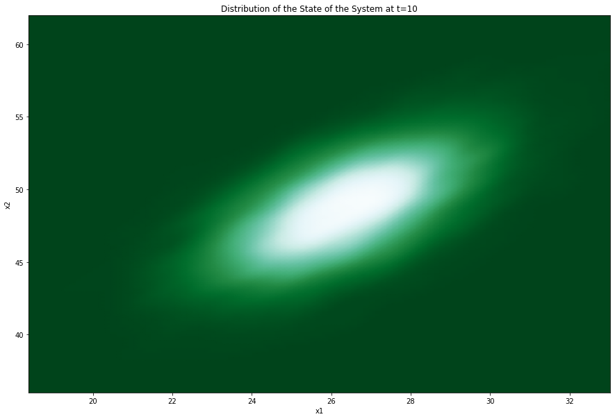
Above we can see the propagated distribution of the state of the system to time $t=10$. We observe that the mean of the population has gone down over time as the supply of food and the overpopulation cannot support the initial population of 100. Similarly, we observe that the mean supply of food has also gone down due to initially high population. Next we are going to plot the time series of mean of population and of food supply over time.

x = np.arange(0, 11, 1)
mean_population = np.array(means)[:, 0]
mean_food_supply = np.array(means)[:, 1]
fig = plt.figure(figsize=(15, 10))
plt.plot(x, mean_population, color="olive", marker="o", markersize=10, linewidth=4, label="Population Mean")
plt.plot(x, mean_food_supply, color="green", marker="o", markersize=10, linewidth=4, label="Food Supply Mean")
plt.xlabel("Time")
plt.ylabel("State")
plt.legend()
plt.title("Means of Population and Food Supply")

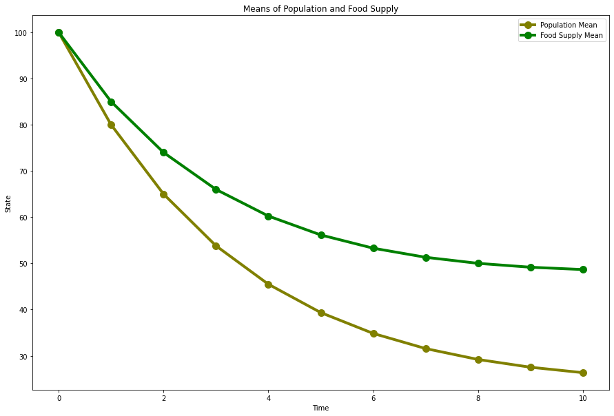
We can see that the initial changes in the expectations of both population and food supply were rapid. However, as time goes, the system tends to an equilibrium point, i.e. such values for population and food supply that can sustain for a long period of time.

Least Squares Estimation

In this section, we are going to discuss how we can update our knowledge of some unknown quantity if we are given measurements. Consider some random vector $\boldsymbol{x}$ that we do not directly observe. Instead, we can only see measurements $\boldsymbol{y}$. We assume the following relationship between the unknown quantity and the measurements:

\[\begin{align*} y_1 &= H_{11}x_1 + H_{12}x_2 + ... + H_{1m}x_m + v_1\\ y_2 &= H_{21}x_1 + H_{22}x_2 + ... + H_{2m}x_m + v_2\\ &\vdots \\ y_n &= H_{n1}x_1 + H_{n2}x_2 + ... + H_{nm}x_m + v_n, \end{align*}\]

where $\boldsymbol{v}$ represents the measurement noise. We know that the variance of each $v_i$ is the same. The above can be expressed in matrix form as

\[\begin{equation*} \boldsymbol{y} = H\boldsymbol{x} + \boldsymbol{v}. \end{equation*}\]

The question that we are interested in is: Given $\boldsymbol{y}$, what is our “best” estimate, $\boldsymbol{\hat{x}}$, of the unknown quantity $\boldsymbol{x}$? Let

\[\begin{equation*} \boldsymbol{e} = \boldsymbol{y} - H\boldsymbol{\hat{x}} \end{equation*}\]

represent the residual, i.e. the difference between the actual measurement and our estimate of the measurement. Provided that we want our estimate to be the one that reduces the squared differences, the cost function $J$ that we want to minimize is of the following form:

\[\begin{align*} J &= e_1^2 + e_2^2 + ... + e_n^2 \\ &= \boldsymbol{e}^T\boldsymbol{e} \\ &= \left(\boldsymbol{y} - H\boldsymbol{\hat{x}}\right)^T \left(\boldsymbol{y} - H\boldsymbol{\hat{x}}\right) \\ &= \boldsymbol{y}^T\boldsymbol{y} - \boldsymbol{\hat{x}}^TH^T\boldsymbol{y} - \boldsymbol{y}^TH\boldsymbol{\hat{x}} + \boldsymbol{\hat{x}}^TH^TH\boldsymbol{\hat{x}} \end{align*}\]

To minimize the error, we need to find the derivative of the cost function with respect to $\boldsymbol{\hat{x}}$. In other words,

\[\begin{equation*} \frac{\partial J}{\partial\boldsymbol{\hat{x}}} = -H^T\boldsymbol{y} - H^T\boldsymbol{y} + 2H^TH\boldsymbol{\hat{x}}. \end{equation*}\]

Set the derivative to zero and solve for $\boldsymbol{\hat{x}}$.

\[\begin{align*} -H^T\boldsymbol{y} - H^T\boldsymbol{y} + 2H^TH\boldsymbol{\hat{x}} &= 0 \\ H^TH\boldsymbol{\hat{x}} &= H^T\boldsymbol{y}\\ \boldsymbol{\hat{x}} &=\left(H^TH\right)^{-1}H^T\boldsymbol{y}. \end{align*}\]

Weighted Least Squares Estimation

In the preceding derivation we assumed that each measurement $y_i$ is equally precise. In other words, we trust each measurement equally. However, in practice, this is not always the case. For example, suppose that you are trying to get the current temperature and you have two measuring devices: thermometer and thermocouple. The latter gives a more precise measurement. One could completely rely on the measurement from the second device. However, instead of completely ignoring the results of the less precise instrument, it would not hurt to include its measurements as well albeit giving it less weight.

We have a similar set-up as in the previous section, i.e.

\[\begin{equation*} \boldsymbol{y} = H\boldsymbol{x} + \boldsymbol{v}. \end{equation*}\]

However, we allow the variance of each of the measurement errors to vary. What we mean is that

\[\begin{equation*} E\left[v_i^2\right] = \sigma_i^2 \end{equation*}\]

may be different for each $i$ and $j$, $i \ne j$. The covariance matrix of the measurement errors is

\[\begin{align*} R &= E\left[\boldsymbol{v}^T\boldsymbol{v}\right]\\ &= \left(\begin{matrix} \sigma_1^2 & 0 & \cdots & 0 \\ 0 & \sigma_2^2 & \cdots & 0\\ \vdots &\vdots & \ddots & \vdots \\ 0 & 0 & \cdots & \sigma_n^2 \end{matrix}\right). \end{align*}\]

The cost function that we want to minimize is of the following form now

\[\begin{align*} J &= \frac{e_1^2}{\sigma_1^2} + \frac{e_2^2}{\sigma_2^2} + \cdots + \frac{e_n^2}{\sigma_n^2} \\ &= \boldsymbol{e}^TR^{-1}\boldsymbol{e} \\ &= \left(\boldsymbol{y} - H\boldsymbol{\hat{x}}\right)^T R^{-1}\left(\boldsymbol{y} - H\boldsymbol{\hat{x}}\right)\\ &= \boldsymbol{y}^TR^{-1}\boldsymbol{y} - \boldsymbol{\hat{x}}^TH^TR^{-1}\boldsymbol{y} - \boldsymbol{y}^TR^{-1}H\boldsymbol{\hat{x}} + \boldsymbol{\hat{x}}^TH^TR^{-1}H\boldsymbol{\hat{x}}. \end{align*}\]

Find the partial derivatives of $J$ with respect to $\boldsymbol{\hat{x}}$.

\[\begin{equation*} \frac{\partial J}{\partial \boldsymbol{\hat{x}}} = -H^TR^{-1}\boldsymbol{y} - H^T\left(R^{-1}\right)^T\boldsymbol{y} + 2H^TR^{-1}H\boldsymbol{\hat{x}}. \end{equation*}\]

Since $R$ is a square diagonal matrix,

\[\begin{equation*} \frac{\partial J}{\partial \boldsymbol{\hat{x}}} = -2H^TR^{-1}\boldsymbol{y} + 2H^TR^{-1}H\boldsymbol{\hat{x}}. \end{equation*}\]

Setting to zero, we get

\[\begin{align} H^TR^{-1}H\hat{\boldsymbol{x}} &= H^TR^{-1}\boldsymbol{y} \nonumber \\ \hat{\boldsymbol{x}} &= \left(H^TR^{-1}H\right)^{-1}H^TR^{-1}\boldsymbol{y}. \label{eq:weighted_OLS_update} \end{align}\]

Recursive Least Squares Estimation

Suppose now that we are getting measurements about a system continuously over time. To implement the methodology explained above, we would have to redo the calculations as per Equation $\left(\ref{eq:weighted_OLS_update}\right)$ each time we get updated measurements. Depending on how often and how many measurements are taken, it may require a lot of computational resources. It would be a good idea if we could somehow incorporate the information from new measurements consequentially, as it becomes available.

Let $\boldsymbol{\hat{x_{n-1}}}$ be our estimate of the random vector $\boldsymbol{x}$ after incorporating measurements $y_1$ to $y_{n-1}$. Next we receive a new measurement $y_n$. How can we incorporate this new information to update our current estimate? The recursive estimator can be written in the following form:

\[\begin{equation} \hat{\boldsymbol{x}}_n = \hat{\boldsymbol{x}}_{n-1} + K_n\left(y_n - H_n\hat{\boldsymbol{x}}_{t-1}\right), \label{eq:state_update} \end{equation}\]

where

\[\begin{equation} y_n = H_n\boldsymbol{x} + v_n \label{eq:measurement_model} \end{equation}\]

and $K_n$ is the estimator gain. We need to find the optimal matrix $K_n$. Let

\[\begin{equation*} \boldsymbol{\epsilon}_n = \boldsymbol{x} - \hat{\boldsymbol{x}}_n \end{equation*}\]

denote the error of the recursive estimate. The expected error is

\[\begin{align*} E\left[\boldsymbol{\epsilon}_n\right] &= E\left[\boldsymbol{x} - \hat{\boldsymbol{x}}_{n-1} - K_n\left(y_n - H_n\hat{\boldsymbol{x}}_{n-1}\right)\right] \\ &= E\left[\boldsymbol{x} - \hat{\boldsymbol{x}}_{n-1} - K_n\left(H_n\boldsymbol{x} + v_n - H_n\hat{\boldsymbol{x}}_{n-1}\right)\right]\\ &= E\left[\boldsymbol{x} - \hat{\boldsymbol{x}}_{n-1} - K_nH_n\boldsymbol{x} + K_nH_n\hat{\boldsymbol{x}}_{n-1} - K_nv_n\right] \\ &= E\left[\left(I- K_nH_n\right)\left(\boldsymbol{x} - \hat{\boldsymbol{x}}_{n-1}\right) - K_nv_n\right] \\ &= \left(I- K_nH_n\right)E\left[\left(\boldsymbol{x} - \hat{\boldsymbol{x}}_{n-1}\right)\right] - K_nE\left[v_n\right]. \end{align*}\]

We observe that if the measurement errors are indeed zero-mean and the initial estimate $\hat{\boldsymbol{x}}_0$ was set to be equal to $E\left[\boldsymbol{x}\right]$, then the expected error is equal to 0, i.e. our estimator is efficient. In that case, the value of the estimator gain $K_n$ does not matter. However, we can use a different metric to find the optimal $K_n$. For example, we could search for such an estimator gain matrix that minimizes the sum of variances of the errors. The cost function is

\[\begin{align*} J_n &= E\left[\left(x_1 - \hat{x}_{n,1}\right)^2 + \left(x_2 - \hat{x}_{n,2}\right)^2 + \cdots + \left(x_m - \hat{x}_{n,m}\right)^2\right] \\ &= E\left[\boldsymbol{\epsilon}_n^T\boldsymbol{\epsilon}_n\right] \\ &= E\left[Tr\left(\boldsymbol{\epsilon}_n\boldsymbol{\epsilon}_n^T\right)\right] \\ &= Tr\left(P_n\right), \end{align*}\]

where $P_n$ is the estimation-error covariance.

\[\begin{align} P_n &= E\left[\left(\left(I- K_nH_n\right)\left(\boldsymbol{x} - \hat{\boldsymbol{x}}_{n-1}\right) - K_nv_n\right)\left(\left(I- K_nH_n\right)\left(\boldsymbol{x} - \hat{\boldsymbol{x}}_{n-1}\right) - K_nv_n\right)^T\right] \nonumber \\ &= E\left[\left(I-K_nH_n\right)\boldsymbol{\epsilon}_{n-1}\boldsymbol{\epsilon}_{n-1}^T\left(I-K_nH_n\right)^T - \left(I-K_nH_n\right)\boldsymbol{\epsilon}_{n-1} v_n^TK_n^T - K_nv_n\boldsymbol{\epsilon}_{n-1}^T\left(I-K_nH_n\right)^T + K_nv_nv_n^TK_n^T\right] \nonumber \\ &= \left(I-K_nH_n\right)P_{n-1}\left(I-K_nH_n\right)^T + K_nR_nK_n^T \label{eq:error_covar_update} \end{align}\]

Equation $\left(\ref{eq:error_covar_update}\right)$ tells us how the estimation-error covariance propagates through time.

Now differentiate the cost function with respect to $K_n$.

\[\begin{align*} \frac{\partial J_n}{\partial K_n} = -2\left(I-K_nH_n\right)P_{n-1}H_n^T + 2K_nR_n. \end{align*}\]

Set equal to 0 and solve for $K_n$.

\[\begin{align} K_nR_n + K_nH_nP_{n-1}H_n^T &= P_{n-1}H_n^T \nonumber \\ K_n\left(R_n + H_nP_{n-1}H_n^T\right) &= P_{n-1}H_n^T \nonumber \\ K_n &= P_{n-1}H_n^T\left(R_n + H_nP_{n-1}H_n^T\right)^{-1}. \label{eq:optimal_gain} \end{align}\]

Equation $\left(\ref{eq:optimal_gain}\right)$ gives us the form of the optimal estimator gain.

Discrete-time Kalman Filter Algorithm

Having provided some essential mathematical background, we are ready to introduce the main topic of this article. In particular, we are going to discuss a discrete-time Kalman filter. Consider a discrete-time dynamical system as in Equation $\left(\ref{eq:linear_system}\right)$ coupled with the measurement model as per Equation $\left(\ref{eq:measurement_model}\right)$.

\[\begin{align*} \boldsymbol{x}_t &= F_{t-1}\boldsymbol{x}_{t-1} + G_{t-1}\boldsymbol{u}_{t-1} + \boldsymbol{w}_{t-1}, \\ \boldsymbol{y}_t &= H_t\boldsymbol{x}_t + \boldsymbol{v}_t, \end{align*}\]

where $\boldsymbol{w}_t \sim N\left(\boldsymbol{0}, Q_t\right)$ and $\boldsymbol{v}_t \sim N\left(\boldsymbol{0}, R_t\right)$ are independent noise vectors. Our aim is to estimate the state of the system using our knowledge of the dynamics of the system and periodic measurements taken.

We already know how the expectation and variance-covariance matrix associated with a linear dynamical system evolve over time. To remind you, they are governed by Equations $\left(\ref{eq:mean_propagation}\right)$ and $\left(\ref{eq:variance_propagation}\right)$. Let $\hat{\boldsymbol{x}}_t^-$ denote our estimate of the state of the system before taking into account the measurement $\boldsymbol{y}_t$ and $\hat{\boldsymbol{x}}_t^+$ denote our estimate after adjusting the estimate by incorporating information from the observation.. Then,

\[\begin{equation} \hat{\boldsymbol{x}}_t^- = F_{t-1}\hat{\boldsymbol{x}}_{t-1}^+ + G_{t-1}\boldsymbol{u}_{t-1}. \label{eq:prediction_step1} \end{equation}\]

The corresponding variance update becomes

\[\begin{equation} P_t^- = F_{t-1}P_{t-1}^+F_{t-1}^T + Q_{t-1}, \label{eq:prediction_step2} \end{equation}\]

where, naturally, $P_{t}^{-}$ is our uncertainty about the state of the system before taking $\boldsymbol{y_t}$ into account, and $P_{t-1}^+$ is our updated uncertainty.

How do we update our estimates by incorporating information from the measurement model? We use the results we developed in the previous section. In particular, the optimal gain is given by

\[\begin{equation} K_t = P_t^-H_t^T\left(R_t + H_tP_t^-H_t^T\right)^{-1}. \label{eq:update_step1} \end{equation}\]

The updated estimates for the state of the system and the corresponding variance-covariance matrix are updated as follows:

\[\begin{equation} P_{t}^+ = \left(I-K_tH_t\right)P_t^-\left(I-K_tH_t\right)^T + K_tR_tK_t^T \label{eq:update_step2} \end{equation}\]

and

\[\begin{equation} \hat{\boldsymbol{x}}_t^+ = \hat{\boldsymbol{x}}_t^- + K_t\left(\boldsymbol{y}_t - H_t\hat{\boldsymbol{x}}_t^-\right). \label{eq:update_step3} \end{equation}\]

Conclusion

When divided into constituent parts, the Kalman filter algorithm is simple and has a very intuitive interpretation to it. Applying the algorithm consequentially in time allows us to get a more precise estimate of the state of dynamically developing systems.

References

1. Simon, D., 2006. Optimal State Estimation. Hoboken, N.J.: Wiley-Interscience.