Gradient Ascent Algorithm

According to Wikipedia, gradient descent (ascent) is a first-order iterative optimization algorithm for finding a local minimum (maximum) of a differentiable function. The algorithm is initialized by randomly choosing a starting point and works by taking steps proportional to the negative gradient (positive for gradient ascent) of the target function at the current point.

The algorithm has a very intuitive interpretation to it as well. One can imagine being placed on some surface with hills and valleys. The elevation represents the value of the function that you want to optimize with respect to. If you want to minimize the function, you want to find the valley with the lowest elevation; similarly, in the case of a maximization problem, you are interested in the hill with the highest elevation. The gradient of the function at the current point identifies the direction of the steepest ascent, i.e. the direction in which the function increases the most at the current point. To illustrate the idea, consider the following function:

\[ F(x,y) = (x^3 + 4y^2) \times \sqrt{|\sin{x^2 + y^2}|}. \]

The 3D plot of the function for \(x \in [-5, 5]\) and \(y \in [-1, 1]\) is shown on Figure 1 below.

Figure 1: 3D Surface Plot for \(F(x,y)\)

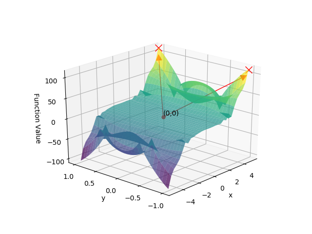
Assuming that we start at point \((0, 0)\) and want to maximize the function, we would be moving in the direction of either of the two points \((4, 1)\) or \((4, -1)\) (the directions are shown as red arrows and the points where the function is maximized are marked by red crosses).

In this post, we will implement gradient ascent for the logistic regression model.

Logistic Regression and Gradient Ascent

The logistic regression is used to model binary outcomes. For example, whether a client of a bank will default within one year. The logistic regression models the probability of \(y=1\) given a vector of explanatory variable \(x\) as

\[ \ln\left(\frac{P(y=1|x)}{1-P(y=1|x)}\right) = x_0 \beta_0 + x_1 \beta_1 + x_2 \beta_2 + … + x_n \beta_n, \]

where \(x_0 = 1\) (this is done to avoid dealing with the intercept term separately). By rearranging the terms, we get

Equation (1) \[ P(y=1|x) = \frac{1}{1 + e^{-(x_0 \beta_0 + x_1 \beta_1 + x_2 \beta_2 + … + x_n \beta_n)}}. \]

The logistic regression model is usually trained using the method of maximum likelihood, i.e. we want to find such parameters \(\beta\) that maximize the likelihood of observing the realizations in the training dataset. The likelihood function for the logistic regression model takes the following form:

Equation (2) \[ L(\beta|y, x) = y^{P(y=1|x)} \times (1-y)^{(1-P(y=1|x))}. \]

However, instead of working with Equation (2) directly, it is more convenient to apply the logarithmic function to get

Equation (3) \[ \text{Log-}L(\beta|y,x) = P(y=1|x) \times \ln y + (1-P(y=1|x)) \times \ln(1-y). \]

The function in Equation 3 is called the log-likelihood function and is much nicer to work with. The optimal set of parameters \(\bar{\beta}\) is then obtained as

\[ \bar{\beta} = argmax_{\beta} \hspace{2mm} \text{Log-}L(\beta|Y,X). \]

To find this optimal set of parameters, we will implement the gradient descent method. The gradient of the log-likelihood function at any point \(x\) is

Equation (4) \[ \nabla \text{Log-}L(\beta|y,x) = \frac{\partial \text{Log-}L(\beta|y,x)}{\partial \beta} = x \times \frac{2y-1}{P(y=1|x)} \times \left(\frac{e^{-(x_0 \beta_0 + x_1 \beta_1 + x_2 \beta_2 + … + x_n \beta_n)}}{(e^{-(x_0 \beta_0 + x_1 \beta_1 + x_2 \beta_2 + … + x_n \beta_n)} + 1)^2} \right). \]

The update rule is then

\[ \beta <= \beta + \alpha \times \nabla \text{Log-}L(\beta|y,x), \]

where \(\alpha\) > 0 is a step size or learning rate (note that by setting \(\alpha < 0\) we are implementing gradient descent instead).

Python Implementation

In this section, we will implement the methodology just explained in Python. We will need the following libraries.

import numpy as np
from sklearn.model_selection import train_test_split
from sklearn.datasets import make_classification
from sklearn.linear_model import LogisticRegression
from sklearn.metrics import accuracy_score
import matplotlib.pyplot as plt

Using make_classification functionality of scikit-learn library, we create a binary classification problem with 1,000 observations. For the sake of simplicity and to make visualizations possible, we only have two independent variables and will not use an intercept term. We leave 20% of the generated data for the test sample.

X, y = make_classification(1000, n_features=2, n_informative=2, n_redundant=0, n_repeated=0, flip_y=0.05, random_state=4)
X_train, X_test, y_train, y_test = train_test_split(X, y, test_size=0.2, random_state=4)

We use the standard normal distribution as the prior distribution of the parameters of the logistic regression model. This way we introduce the least amount of bias into our analysis. Note, however, that if an analyst has some knowledge of the problem at hand, he might be smart about how he initializes the parameters to speed up the algorithm and make it less likely to get stuck in some local maximum (minimum) which is not the global maximum (minimum) of the target function.

np.random.seed(4)
W = np.random.randn(2)

The code snippet below implements Equation (1), i.e. it outputs the probability of \(y=1\).

def predict(x, w):
    return 1 / (1 + np.exp(-np.matmul(x, w)))

For example, the probability that the first observation in the training dataset belongs to class 1 is 74.31%.

predict(X_train[0], W)

0.7431

Let us estimate the overall accuracy of our model on the training dataset.

predictions = predict(X_train, W)
predictions = predictions.astype(int)
accuracy_score(y_train, predictions)

0.5025

As expected, the accuracy is around 50%. In other words, our model is no better than random guessing at this point. We will compare the accuracy of the trained model to see if our implementation of the gradient ascent method has been successful.

Next we define estimate_gradient function that is the implementation of Equation (4).

def estimate_gradient(x, y, w):
    return np.nan_to_num((2 * y - 1) / predict(x, W) * x * np.nan_to_num(np.exp(-np.matmul(x, w))) / (np.nan_to_num(np.exp(-np.matmul(x, w))) + 1)**2)

We set the learning rate to be equal to 0.0005 and the number of epochs, i.e. the number of times we will be going over the training dataset, to be 45.

a = 0.005
num_epochs = 45

Finally, the code snippet below implements the gradient ascent algorithm we discussed in the previous section. Note that we save the accuracies which we will use further for the contour plot.

parameter_values = np.reshape(W, (1, -1))
accuracy_ratios = [accuracy_score(y_train, predictions)]
for i in range(num_epochs):
    for j in range(X_train.shape[0]):
        W = W + a * estimate_gradient(X_train[j], y_train[j], W)
    parameter_values = np.concatenate((parameter_values, np.reshape(W, (1, -1))), axis=0)
    predictions = predict(X_train, W)
    predictions = predictions.astype(int)
    accuracy_ratios.append(accuracy_score(y_train, predictions))

The training is over and we can check the performance of the model on the training dataset.

predictions = predict(X_train, W)
predictions = predictions.astype(int)
accuracy_score(y_train, predictions)

0.8375

As can be seen, the model now achieves an accuracy ratio of 83.75% which is a significant improvement over the performance achieved by the untrained model. To make sure that our implementation did not lead to any overfitting, we are checking the accuracy ratio on the test set that was not used in training.

predictions = predict(X_test, W)
predictions = predictions.astype(int)
accuracy_score(y_test, predictions)

0.83

The accuracy ratio of 83% on the test set is close to the one achieved on the training set and we may conclude that the model indeed learned some useful information about the relationships between the target variable and the two explanatory variables.

Finally, we are going to create a contour plot of accuracy ratio as a function of different sets of parameters \(\beta\). Simply put, contour plots allow us to show 3D surfaces on a 2D plane.

X, Y = np.meshgrid(parameter_values[:, 0], parameter_values[:, 1])
Z = np.zeros((X.shape[0], X.shape[1]))
for i in range(X.shape[0]):
    for j in range(X.shape[1]):
        w = np.array([X[1][j], Y[i][1]])
        predictions = predict(X_train, w)
        predictions = predictions.astype(int)
        Z[i][j] = accuracy_score(y_train, predictions)
plt.contourf(X, Y, Z, 15, cmap='RdGy')
plt.xlabel('Beta1')
plt.ylabel('Beta2')
plt.colorbar();

Figure 2: Accuracy Ratio Contour Plot

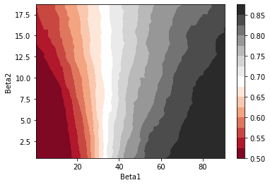
The areas of the same color on the contour plot tell us that we can expect to achieve the same level of prediction accuracy. For example, for \(\beta_2 = 2.5\) and \(\beta_1 >= 70\), we expect to achieve an accuracy of 85% as measured on the training dataset.