Antithetic Variates Method for Variance Reduction in Monte Carlo Simulations

Wikipedia defines Monte Carlo methods as “…a broad class of computational algorithms that rely on repeated random sampling to obtain numerical results.” The three most common applications are: generating draws from a probability distribution, optimization and numerical integration. The latter problem can be expressed as follows:

\[\begin{equation} \int_{a}^{b}g(x)dx, \hspace{2mm} a<b. \end{equation} \label{eq:problem}\]

Depending on how complex the function $g$ is, an analytical solution for $\eqref{eq:problem}$ may or may not be easy to obtain. However, the problem of solving the above integral is equivalent to the problem of evaluating the following expectation:

\[\begin{equation} E\left[g\left(U\right)\right]\times(b-a), \end{equation} \label{eq:expectation_problem}\]

where $U$ is a continuous uniform random variable on $[a, b]$, i.e., $U\sim U_{[a,b]}$. This comes from the fact that

\[\begin{align*} E\left[g\left(U\right)\right] &= \int_{\mathbb{R}}g(x)f(x)dx \\ &= \int_{-\infty}^{a}g(x)f(x)dx + \int_{a}^{b}g(x)f(x)dx + \int_{b}^{\infty}g(x)f(x)dx, \end{align*}\]

where $f$ is the PDF of $U$ given by

\[\begin{equation*} f(x) = \begin{cases} \frac{1}{b-a} \hspace{2mm}\text{for} \hspace{2mm} x \in [a,b]\\ 0 \hspace{9mm}\text{otherwise}. \end{cases} \end{equation*}\]

Therefore,

\[\begin{align*} E\left[g\left(U\right)\right] = \int_{a}^{b}g(x)\frac{1}{b-a}dx = \frac{1}{b-a}\int_{a}^{b}g(x)dx. \end{align*}\]

If we had a random sample of size $n$ of independently and uniformly distributed random variables, $\textbf{U}=(U_1, U_2, …, U_n)$, we could estimate the expectation in $\eqref{eq:expectation_problem}$ with the help of the sample mean:

\[\begin{equation*} \hat{\mu} = \frac{1}{n}\sum_{i=1}^{n}g\left(U_i\right). \end{equation*}\]

The corresponding standard error of the mean would be:

\[\begin{equation} SE(\hat{\mu}) = \frac{\sigma}{\sqrt{n}}, \label{eq:se} \end{equation}\]

where

\[\begin{equation*} \sigma = E\left[\left(g(U) - E\left[g(U)\right]\right)^2\right]. \end{equation*}\]

Of course, to make our estimate more precise, we are are interested in reducing $SE(\hat{\mu})$. The straightforward approach is to increase the size of the random sample, $n$. However, since the standard error has a one over square root convergence, to reduce the standard error by a factor of 10, we would need to increase the sample size by a factor of 100. Therefore, depending on how small we require the standard error to be, we may need a lot of computational power to run the required number of Monte Carlo simulations. Variance reduction techniques, like antithetic variate approach, aim to reduce the standard error by reducing $\sigma$ in $\eqref{eq:se}$ instead.

Antithetic Variates

As mentioned previously, the antithetic variates method is a variance reduction technique. For each random variable $g(U_i)$, the key idea is to take its antithetic variate, $\tilde{g(U_i)}$, so that

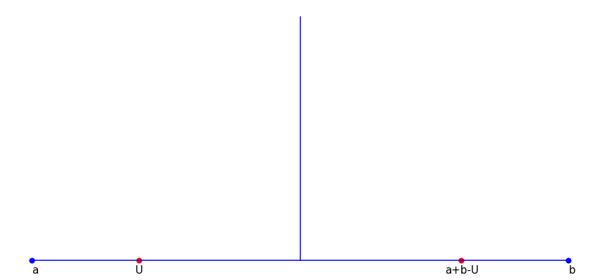
\[\begin{equation} \frac{1}{n}\sum_{i=1}^{n/2}g(U_i)+\tilde{g(U_i)}, \hspace{2mm} n=2m, \hspace{2mm} m \in \mathbb{N} \end{equation}\]

is still an unbiased estimate of $E\left[g(U)\right]$. In the case of uniformly distributed random variables, i.e., $U_i\sim U_{[a,b]}$, we can set $\tilde{g(U_i)}=g(a+b-U_i)$. In other words, the antithetic variate is the function $g$ applied to the reflection of $U_i$ through the center point (see Figure 1 below).

Figure 1. Reflection of a Point through the Center Point

The corresponding variance of the sample mean becomes:

\[\begin{align*} Var\left(\frac{1}{n}\sum_{i=1}^{n/2}g(U_i)+\tilde{g(U_i)}\right) &= \frac{1}{n^2}\sum_{i=1}^{n/2}\sum_{j=1}^{n/2}Cov\left(g(U_i) + g\left(a+b-U_i\right), g(U_j) + g\left(a+b-U_j\right)\right) \\ &= \frac{1}{n^2}\sum_{i=1}^{n/2}Var\left(g(U_i) + g\left(a+b-U_i\right)\right) \\ &= \frac{1}{n^2}\sum_{i=1}^{n/2}Var\left(g(U_i)\right) + Var\left(g\left(a+b-U_i\right)\right) + 2Cov\left(g(U_i), g\left(a+b-U_i\right)\right)\\ &= \frac{1}{n^2}\sum_{i=1}^{n/2}2Var\left(g(U_i)\right) + 2Cov\left(g(U_i), g\left(a+b-U_i\right)\right)\\ &= \frac{1}{n^2}\sum_{i=1}^{n/2}2Var\left(g(U_i)\right) + 2Corr\left(g(U_i), g\left(a+b-U_i\right)\right)\times \sqrt{Var\left(g(U_i)\right)} \times \sqrt{Var\left(g\left(a+b-U_i\right)\right)}\\ &= \frac{1}{n^2}\sum_{i=1}^{n/2}2Var\left(g(U_i)\right) + 2Corr\left(g(U_i), g\left(a+b-U_i\right)\right)\times Var\left(g(U_i)\right)\\ &= \frac{2\sigma}{n^2}\sum_{i=1}^{n/2}\left(1+\rho\right)\\ &= \frac{\sigma}{n}\left(1+\rho\right), \end{align*}\]

where we used the fact that $U_i, U_2,…,U_{n/2}$ is a sequence of independent random variables and that if $U_i\sim U_{[a,b]}$, so does $\left(a+b-U_i\right)$. Therefore,

\[\begin{align*} -1 &\le \rho \le 1 \\ 0 &\le 1 + \rho \le 2 \\ 0 & \le \frac{\sigma}{n}\left(1 + \rho \right) \le \frac{2\sigma}{n}. \end{align*}\]

The above implies that the antithetic variates method can reduce the variance of the sample mean to 0 or double the variance of the plain vanilla Monte Carlo simulation approach. It all depends on $\rho$: if $\rho<0$, then the antithetic variate method reduces the standard error of the mean; if $\rho > 0$, the antithetic variate technique increases the standard error of the mean. In the case of uniformly distributed random variables, monotonicity of the function $g$ guarantees that $\rho \le 0$.

Proposition. Suppose $U\sim U_{[a,b]}$ and $g$ is monotone. Then, $Corr\left(g(U), g\left(a+b-U\right)\right) \le 0$.

Proof. Without loss of generality, suppose $g$ is monotonically increasing, i.e., $g(x)\le g(y)$ whenever $a\le x\le y\le b$. We need to show that $Cov\left(g(U), g\left(a+b-U\right)\right) \le 0$. We have:

\[\begin{align*} Cov\left(g(U), g\left(a+b-U\right)\right) &= E\left[\left(g(U) - E[g(U)]\right)\left(g\left(a+b-U\right) - E\left[g\left(a+b-U\right)\right]\right)\right] \\ &= E\left[(g(U) - \mu)\left(g\left(a+b-U\right) - \mu\right)\right] \\ &= \int_{a}^{b}(g(x)-\mu)\left(g\left(a+b-x\right) - \mu\right)f(x)dx \\ &= \frac{1}{b-a}\int_{a}^{b}(g(x)-\mu)\left(g\left(a+b-x\right) - \mu\right)dx. \end{align*}\]

Let $x\in[a,b]$ be arbitrary. If $x\le\frac{a+b}{2}$, then $g(x)\le \mu$ due to monotonicity of $g$. Moreover, if $x\le\frac{a+b}{2}$, then $a+b-x\ge \frac{a+b}{2}$. Consequently, $g(a+b-x) \ge \mu$. It follows that $(g(x)-\mu)\left(g\left(a+b-x\right) - \mu\right) \le 0$. Similarly, we can show that if $x > \frac{a+b}{2}$, then $(g(x)-\mu)\left(g\left(a+b-x\right) - \mu\right) \le 0$. Thus,

\[\begin{equation*} Cov\left(g(U), g\left(a+b-U\right)\right) = \frac{1}{b-a}\int_{a}^{b}(g(x)-\mu)\left(g\left(a+b-x\right) - \mu\right)dx \le 0. \\ \hspace{200mm}\blacksquare \end{equation*}\]

Numerical Example

Suppose we want to estimate the following integral using the Monte Carlo method:

\[\int_{0}^{1}\frac{1}{1+x}dx.\]

The exact result is

\[\int_{0}^{1}\frac{1}{1+x}dx = \ln(2) \approx 0.6931471805599453.\]

Expressing the problem via a uniformly distributed random variable $U \sim U_{[0,1]}$,

\[\int_{0}^{1}\frac{1}{1+x}dx = E\left[\frac{1}{1+U}\right].\]

We can generate 3,000 samples from $U_{[0,1]}$ and obtain a numerical estimate as follows.

import numpy as np
import time

np.random.seed(4)
n = 3000
start_time = time.perf_counter()
x = np.random.uniform(size=n)
y = 1 / (1+x)
print("The estimate is ", np.mean(y))
print("Time taken: ", time.perf_counter() - start_time, " seconds")
print("The standard error is ", np.sqrt(np.var(y, ddof=1)/n));

The estimate is  0.6918232680515748
Time taken:  0.0006878439962747507  seconds
The standard error is  0.0025820198681014237

Since $g$ is monotone, we know that the antithetic variates method is likely to yield positive results, i.e., lower standard error. The code snippet below implements this method.

np.random.seed(4)
m = int(n / 2)
start_time = time.perf_counter()
x = np.random.uniform(size=m)
x_antithetic = 1 - x
y = 1 / (1 + x)
y_antithetic = 1 / (1 + x_antithetic)
print("The estimate is ", np.mean((y + y_antithetic) / 2))
print("Time taken: ", time.perf_counter() - start_time, " seconds")
print("The standard error is ", np.sqrt(np.var((y + y_antithetic) / 2, ddof=1) / m ));

The estimate is  0.6935171099447586
Time taken:  0.0006737630028510466  seconds
The standard error is  0.0006373082743002956

With around the same time taken, using the antithetic variate method, we obtained a slightly more accurate estimate. Furthermore, we managed to reduce the standard error by a factor of about 4. That is,

\[\begin{equation*} \frac{0.0025820198681014237}{0.0006373082743002956} \approx 4.05 \end{equation*}\]

Given the one over square root relationship between the standard error and the sample size as per Equation $\eqref{eq:se}$, to reduce the standard error of the plain vanilla implementation of the Monte Carlo method, we would need to increase the sample size by a factor of 16 as demonstrated by the following code.

np.random.seed(4)
n = 3000 * 16
start_time = time.perf_counter()
x = np.random.uniform(size=n)
y = 1 / (1+x)
print("The estimate is ", np.mean(y))
print("Time taken: ", time.perf_counter() - start_time, " seconds")
print("The standard error is ", np.sqrt(np.var(y, ddof=1)/n));

The estimate is  0.6931998818943664
Time taken:  0.0020677989959949628  seconds
The standard error is  0.0006420798804208894

As a direct consequence of a larger sample used in the plain vanilla implementation, the estimation time is increased by a factor of 3, i.e.,

\[\begin{equation*} \frac{0.0020677989959949628}{0.0006878439962747507} \approx 3 \end{equation*}\]

The table below summarizes the results of the three simulations.

Table 1. Comparison of Plain Vanilla MC Implementation and Antithetic Variates Method

Monte Carlo Method	Sample Size	Standard Error	Time Spent (seconds)
Plain Vanilla	3,000	0.0025820198681014237	0.0006878439962747507
Plain Vanilla	48,000	0.0006420798804208894	0.0020677989959949628
Antithetic Variates	3,000	0.0006373082743002956	0.0006737630028510466

Summing up, the antithetic variates technique is a simple way to improve estimates from Monte Carlo simulations.