Abalone. Part 2
This is the second part for the project about constructing a predictive model for the abalone dataset. In this post, we are going to fit 3 different regression algorithms and see which one of them performs best on our dataset.
For those who would like to follow along, we would require the following Python libraries:
import pandas as pd
import numpy as np
import matplotlib.pyplot as plt
from IPython.display import IFrame
from sklearn.model_selection import train_test_split
from sklearn.model_selection import GridSearchCV
from sklearn.linear_model import LinearRegression
from sklearn.neighbors import KNeighborsRegressor
from sklearn.ensemble import RandomForestRegressor
We will directly upload the dataset that we cleansed in the previous post.
dataset = pd.read_csv('clean_data', index_col=0)
dataset.head()
| sex_F | sex_I | sex_M | length | diameter | height | whole_weight | shucked_weight | viscera_weight | shell_weight | rings | |
|---|---|---|---|---|---|---|---|---|---|---|---|
| 0 | 0 | 0 | 1 | 0.455 | 0.365 | 0.095 | 0.5140 | 0.2245 | 0.1010 | 0.150 | 15 |
| 1 | 0 | 0 | 1 | 0.350 | 0.265 | 0.090 | 0.2255 | 0.0995 | 0.0485 | 0.070 | 7 |
| 2 | 1 | 0 | 0 | 0.530 | 0.420 | 0.135 | 0.6770 | 0.2565 | 0.1415 | 0.210 | 9 |
| 3 | 0 | 0 | 1 | 0.440 | 0.365 | 0.125 | 0.5160 | 0.2155 | 0.1140 | 0.155 | 10 |
| 4 | 0 | 1 | 0 | 0.330 | 0.255 | 0.080 | 0.2050 | 0.0895 | 0.0395 | 0.055 | 7 |
As a reminder, we previously created 3 dummy variables to represent a categorical variable, sex, with 3 possible values. However, if we proceed this way, we are actually getting into the Dummy Variable Trap, i.e. we are introducing a redundant dummy variable that carries no extra information. This is due to the fact that we only need \(k-1\) dummy variables to represent a categorical variable with \(k\) distinct values. For that reason, we are going to drop sex_F, sex_M and sex_I variables and introduce only 2 dummy variables instead: dummy_sex_1 and dummy_sex_2. We are going to encode information related to sex as follows:
- Male: dummy_sex_1 = 1 and dummy_sex_2 = 1
- Female: dummy_sex_1 = 1 and dummy_sex_2 = 0
- Infant: dummy_sex_1 = 0 and dummy_sex_2 = 0
dataset['dummy_sex_1'] = np.where(dataset.sex_I==1, 0, 1)
conditions = [(dataset['dummy_sex_1']==1) & (dataset['sex_F']==1), (dataset['dummy_sex_1']==1) & (dataset['sex_M']==1)]
choices = [0, 1]
dataset['summy_sex_2'] = np.select(conditions, choices)
Let us see if we correctly introduced the auxiliary dummy variables.
dataset.head()
| sex_F | sex_I | sex_M | length | diameter | height | whole_weight | shucked_weight | viscera_weight | shell_weight | rings | dummy_sex_1 | summy_sex_2 | |
|---|---|---|---|---|---|---|---|---|---|---|---|---|---|
| 0 | 0 | 0 | 1 | 0.455 | 0.365 | 0.095 | 0.5140 | 0.2245 | 0.1010 | 0.150 | 15 | 1 | 1 |
| 1 | 0 | 0 | 1 | 0.350 | 0.265 | 0.090 | 0.2255 | 0.0995 | 0.0485 | 0.070 | 7 | 1 | 1 |
| 2 | 1 | 0 | 0 | 0.530 | 0.420 | 0.135 | 0.6770 | 0.2565 | 0.1415 | 0.210 | 9 | 1 | 0 |
| 3 | 0 | 0 | 1 | 0.440 | 0.365 | 0.125 | 0.5160 | 0.2155 | 0.1140 | 0.155 | 10 | 1 | 1 |
| 4 | 0 | 1 | 0 | 0.330 | 0.255 | 0.080 | 0.2050 | 0.0895 | 0.0395 | 0.055 | 7 | 0 | 0 |
By comparing information contained in the original dummy variables and the newly created ones, we can see that the encoding was done correctly. Thus, we may now drop the original dummy variables.
dataset.drop(['sex_F', 'sex_I', 'sex_M'], axis=1, inplace=True)
When building a predictive model, it is a common practice to split the whole dataset into 3 parts: training, validation and test. Training dataset is used to build a predictive model itself. Validation dataset is used to test and pick the best set of hyperparameters. Finally, test set is used to assess the “real” power of the trained model, i.e. the performance that the model is going to achieve on unseen data. For our purposes, we are going to keep 60% of observations for training purposes, 20% for validation dataset and the remaining 20% as the last test.
train_x, test_x, train_y, test_y = train_test_split(dataset.drop(['rings'], axis=1), dataset.rings, test_size=0.2, random_state=4)
train_x, valid_x, train_y, valid_y = train_test_split(train_x, train_y, test_size=0.25, random_state=8)
The first model that we are going to use is a plain vanilla linear regression model. Since there are no hyperparameters to adjust, we are going to use both training and validation datasets to train the model.
linear_regression = LinearRegression()
linear_regression.fit(train_x.append([valid_x]), train_y.append([valid_y]))
linear_regression.score(train_x.append([valid_x]), train_y.append([valid_y]))
0.5400939011738732
The model achieved an \(R^2\) of 54%, meaning that about 54% of total variation is explained by the model. Before we assess our model’s performance on the test set, let us investigate the coefficients for the predictor variables.
for i, j in zip(dataset.drop(['rings'], axis=1).columns, linear_regression.coef_):
    print(i,': ', np.round(j, decimals=2))
length :  0.3
diameter :  10.82
height :  9.77
whole_weight :  8.63
shucked_weight :  -19.76
viscera_weight :  -10.17
shell_weight :  9.54
dummy_sex_1 :  0.76
summy_sex_2 :  0.09
The signs for most of the coefficients make sense. For example, we can see that abalone age, as represented by rings variable, is expected to rise with length, diameter, height, whole weight, shell weight as well as with the introduced earlier dummy variables. However, according to the model constructed, there is an inverse relationship between shucked weight and age, and viscera weight and age. Unfortunately, there are no experts to consult with about the validity of the estimates for these coefficients. Thus, we will proceed ignoring these facts.
With respect to the dummy variables, since dummy_sex_1 takes a value of 1 only for grown abalone, i.e. both male and female, we can see that its coefficient is higher than that of dummy_sex_2, which only takes value of 1 for grown male abalone.
Finally, we can assess how the constructed linear regression model will perform on unseen data by measuring its \(R^2\) coefficient on the test set.
linear_regression.score(test_x, test_y)
0.5382517042512784
\(R^2\) of 53.8% is very close to the performance shown on the training dataset. Thus, we expect it to be a good indicator of the true predictive power of the model. Also, there was no overfitting on the training dataset.
The next model is k-nearest neighbors regression. This model makes a prediction for the target variable by averaging the values of the target variable of \(k\) closest neighbors. This is a very simple algorithm and only requires a single hyperparameter to tune - the number of neighbors to consider. Thus, we are going to test powers of 2 as the potential values for the number of neighbors.
neighbors = [2 ** i for i in range(1, 7)]
k_neighbors_regressors = [KNeighborsRegressor(n_neighbors=i) for i in neighbors]
validation_scores = [k_neighbors_regressors[i].fit(valid_x, valid_y).score(valid_x, valid_y) for i in range(len(neighbors))]
for i in range(len(neighbors)):
    print("R^2 for regressor with ", neighbors[i], " neighbors is: ", validation_scores[i])
R^2 for regressor with  2  neighbors is:  0.8035060102623917
R^2 for regressor with  4  neighbors is:  0.6885811970171609
R^2 for regressor with  8  neighbors is:  0.609469972657626
R^2 for regressor with  16  neighbors is:  0.5244964524845105
R^2 for regressor with  32  neighbors is:  0.459671963818305
R^2 for regressor with  64  neighbors is:  0.3860593076756865
The best performance on the validation set, with \(R^2\) of about 80%, was achieved by a model with only 2 neighbors. We can also see that the performance tends to decrease as the number of neighbors is increased. The model with 64 neighbors achieved an \(R^2\) of only about 39%.
Next, to test if there was any overfitting on the validation dataset, we are going to measure the performance of all models on the training dataset.
training_scores = [k_neighbors_regressors[i].score(train_x, train_y) for i in range(len(neighbors))]
for i in range(len(neighbors)):
    print("R^2 for regressor with ", neighbors[i], " neighbors is: ", training_scores[i])
R^2 for regressor with  2  neighbors is:  0.3588592806835669
R^2 for regressor with  4  neighbors is:  0.45152448611527707
R^2 for regressor with  8  neighbors is:  0.4901085189740877
R^2 for regressor with  16  neighbors is:  0.4740491034345346
R^2 for regressor with  32  neighbors is:  0.4393814851436775
R^2 for regressor with  64  neighbors is:  0.38530314857839243
Indeed, we observe slightly different results this time. The model with 8 neighbors is the best performer. We may conclude that there was severe overfitting on the validation dataset. The figure below shows how performance of the models constructed differ on the validation and test sets as a function of the number of neighbors.
fig = plt.figure(figsize=(15,8), dpi=100)
ax = fig.add_subplot()
ax.set_xlabel("Number of neigbors")
ax.set_ylabel("R^2")
ax.plot(neighbors, validation_scores, label='Validation sample')
ax.plot(neighbors, training_scores, label='Training sample')
ax.legend(loc='best')
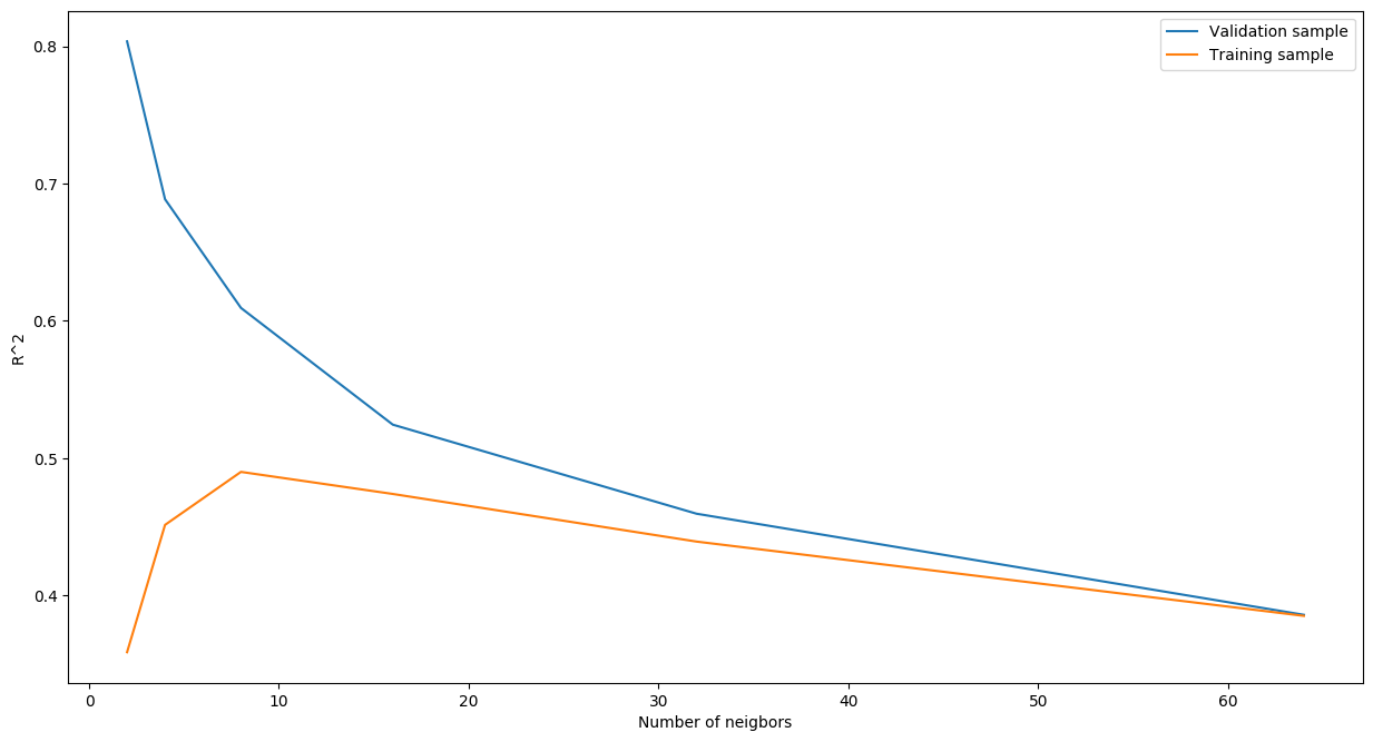
To people familiar with data science, the shape of the above figure should be known. Basically, we can see the trade-off between bias (underfitting) and variance (overfitting). With a very low number of neighbors, our algorithm performs really well on the validation set but severely underperforms on the training set. As the number of neighbors is increased, the performance on the validation dataset keeps on decreasing. However, on the training dataset, it starts to increase up to a point of highest \(R^2\) and then starts to slide down. Hence, we should keep the model that performed the best on the training dataset, i.e. the one with 8 neighbors, re-train it on the training set and check its expected performance on the test set.
k_neighbors_regressor = KNeighborsRegressor(n_neighbors=8)
k_neighbors_regressor.fit(train_x, train_y)
k_neighbors_regressor.score(train_x, train_y)
0.6302705828791839
We obtained an \(R^2\) of 63% on the training dataset. Finally, we are going to test the model on the test set.
k_neighbors_regressor.score(test_x, test_y)
0.5330054277244697
The performance on the test set has dropped down to 53% as compared to the training set. However, we note that the performance is comparable with the performance achieved by the linear regression model.
The last model we are going to use on this dataset is a random forest regression model. This is a model with higher capacity than the models we already considered. In other words, this model is, potentially, better performing and may account for more complex structures of data. However, on the other hand, this model is more prone to overfitting on the training dataset and thus requires careful consideration when it comes to choosing hyperparameters.
We are going to utilize GridSearchCV class of scikit-learn library. This allows us to implement a grid search in the hyperparameter space and obtain the best set of hyperparameters.
parameter_grid = [
    {'max_depth': list(range(3, 8)),
     'max_features': list(range(4, 10)),
     'min_samples_split': [2**i for i in range(1, 5)],
     'min_samples_leaf': [2**i for i in range(1, 5)]
    }
]

reg = RandomForestRegressor()
random_forest_regressor = GridSearchCV(reg, parameter_grid)
random_forest_regressor.fit(train_x.append([valid_x]), train_y.append([valid_y]))
random_forest_regressor = random_forest_regressor.best_estimator_
random_forest_regressor
RandomForestRegressor(bootstrap=True, criterion='mse', max_depth=7,
                      max_features=8, max_leaf_nodes=None,
                      min_impurity_decrease=0.0, min_impurity_split=None,
                      min_samples_leaf=8, min_samples_split=8,
                      min_weight_fraction_leaf=0.0, n_estimators=10,
                      n_jobs=None, oob_score=False, random_state=None,
                      verbose=0, warm_start=False)
We can see that the best performing random forest uses a maximum of 8 features to construct each individual regression tree, it also uses a minimum sample per leaf of 8 and a minimum sample of 8 to split a given node. Also, each forest was constructed by using 10 individual regression trees. Note that GridSearchCV uses cross-validation technique to choose the best performing random forest regressor, we do not need to make a split between training and validation dataset. Instead, we combined them together to obtain the best set of hyperparameters.
Let us now see how well the best model performed on the training dataset.
random_forest_regressor.score(train_x.append([valid_x]), train_y.append([valid_y]))
0.6474251680954815
Similar to k-nearest neighbors regressor, random forest regressor achieved an \(R^2\) of about 65%. However, as we mentioned previously, this algorithms tends to overfit. Thus, we should expect a lower performance on the test set.
random_forest_regressor.score(test_x, test_y)
0.5550481847637081
As expected, the model achieved an \(R^2\) of only 55% on the test set, i.e. a drop of about 10% as compared to the training set. Furthermore, all 3 regression models obtained about the same performance on this dataset. According to Occam’s razor principle, we should go with linear regression model as the simplest among the three. Furthermore, linear regression is not a “black-box” model and we can actually investigate and trace how the model makes its predictions.