Notes on Reinforcement Learning Lectures by David Silver

I have recently finished watching and working through a series of lectures by David Silver on Reinforcement Learning that I found immensely useful. Throughout the course, I have been keeping notes and providing additional clarifications where I thought they could help with the overall understanding of the topic. I am hereby sharing my notes in the hope that people interested in Reinforcement Learning can find something useful for themselves. I do not own the images used in the current post but they were taken directly from the lecture slides by professor David Silver.

Introduction to Reinforcement Learning

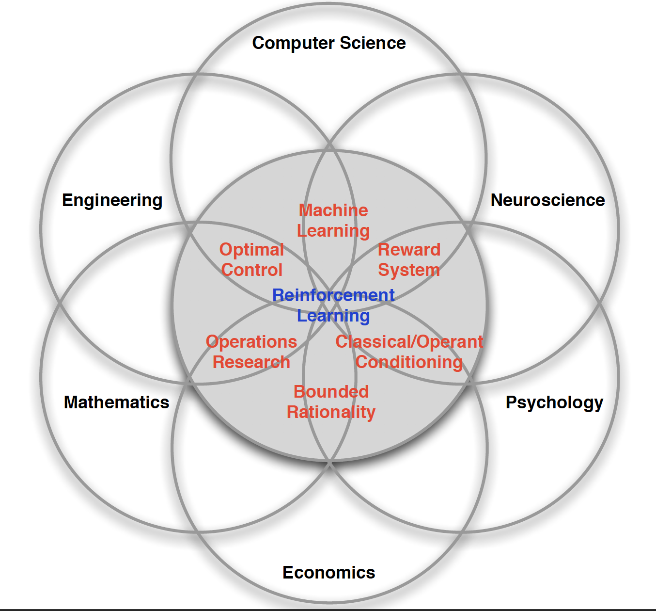
The object studied by RL community is how to make optimal decisions in an environment. Many other disciplines actually study the same problem. For example, in economics, we have agents that want to maximize their utility function (also game theory). In psychology, we study human and animal behavior. In engineering, we have optimal control; in mathematics - operations research.

The main aim of RL is to maximize the sum of future rewards.

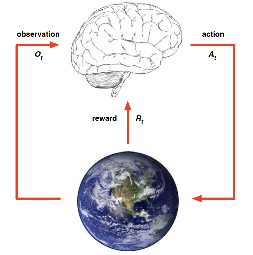
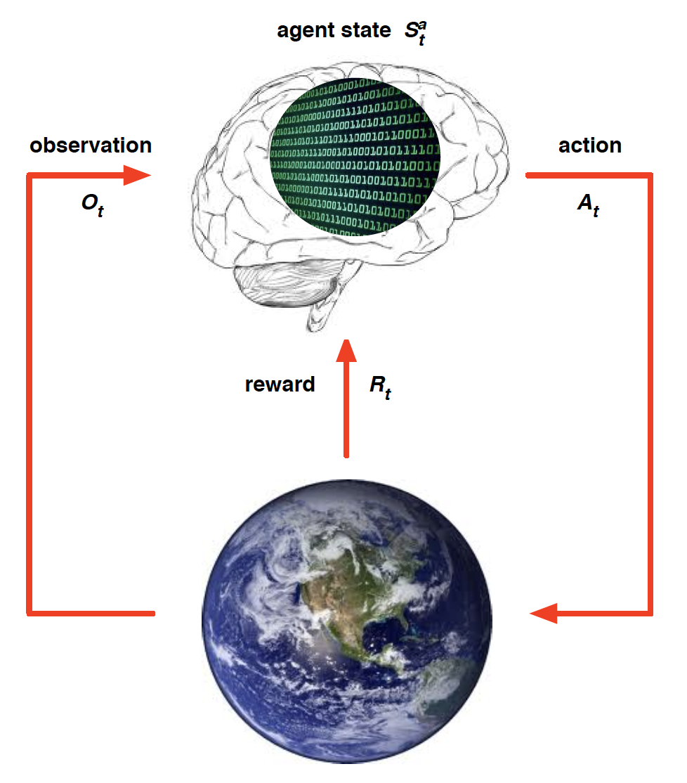
We can think of an RL problem as of building a brain that needs to learn to take optimal actions in an environment. The brain can only affect the environment through actions that it takes. The environment, on the other hand, provides the agent with a reward and an updated observation.

For example, when applied to an Atari game, we would have

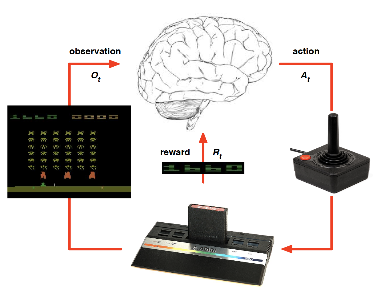
History is everything that the agent has observed/experienced up to time $t$. It includes a sequence of observations, actions and rewards received by the agent.

\[\begin{equation*} H_t = O_1, A_1, R_1, O_2, ..., O_{t-1}, A_{t-1}, R_{t-1}, O_t. \end{equation*}\]

However, for real life problems, it becomes too difficult to keep track of all the history observed by the agent. Instead, we want to come up with a mapping that would summarize the history observed up to some time t. Such a mapping is called “state”.

\[\begin{equation*} S_t = f\left(H_t\right). \end{equation*}\]

Thus, when we talk about the state of the environment, we are talking about a set of numbers that determine what is going to happen next.

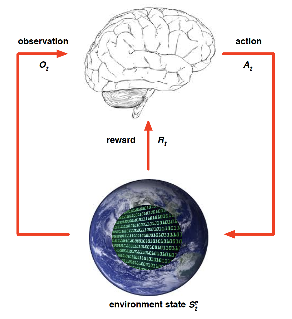
However, in most realistic scenarios, our agent does not get to observe the state of the environment. Instead, he is only looking at the observations spit out by the environment. Consequently, our algorithms cannot depend on the state of the environment.

On the other hand, agent state is all the information that our agent uses to take action.

In a simple case, i.e. the case of full observability, agent directly observes environment state. In other words, agent state = environment state = information state. This leads to a Markov Decision Process (MDP).

Partial observability: agent observes the environment only indirectly. For example, a poker playing agent only observes public cards, i.e. he cannot see what cards other players have. In this case, we would work with Partially Observable Markov Decision Process (POMDP). The agent would have to construct its own state representation.

To summarize observability, consider an agent that needs to learn to play an atari game. This is a partial observability problem because our agent does not get to see the whole state of the environment which is basically all the numbers saved in the console that are used to determine what is going to happen next (think of random seeds, game logic, etc.). Instead, the agent only observes the visual output on the screen.

Similarly, agent state is a set of numbers that summarizes our agent, i.e. what the agent has seen, how he makes his decisions, etc. Unlike the state of the environment, we observe the state of our agent directly. We get to build this state function ourselves.

This is when the notion of Markov state comes into play. Namely, a state $S_t$ is Markov if

\[\begin{equation*} P\left[S_{t+1}|S_t\right] = P\left[S_{t+1}|S_1, S_2,\cdots, S_t\right]. \end{equation*}\]

The Markov property of a system basically says that the future is independent of the past given the present. In other words, if a state is Markov, we can safely discard all the previous information that we observed and just use whatever is in the present. The idea is then that we can work with something much more compact. The state fully characterizes the distribution over all the future actions, observations and rewards. Consider the following example

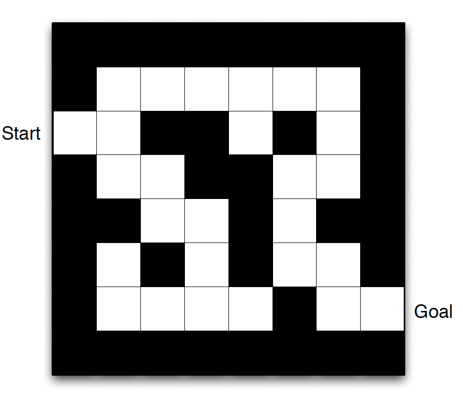
Once we are in a given cell, we do not care where we were before.

What is inside our RL agent? There may be one or more of the following components:

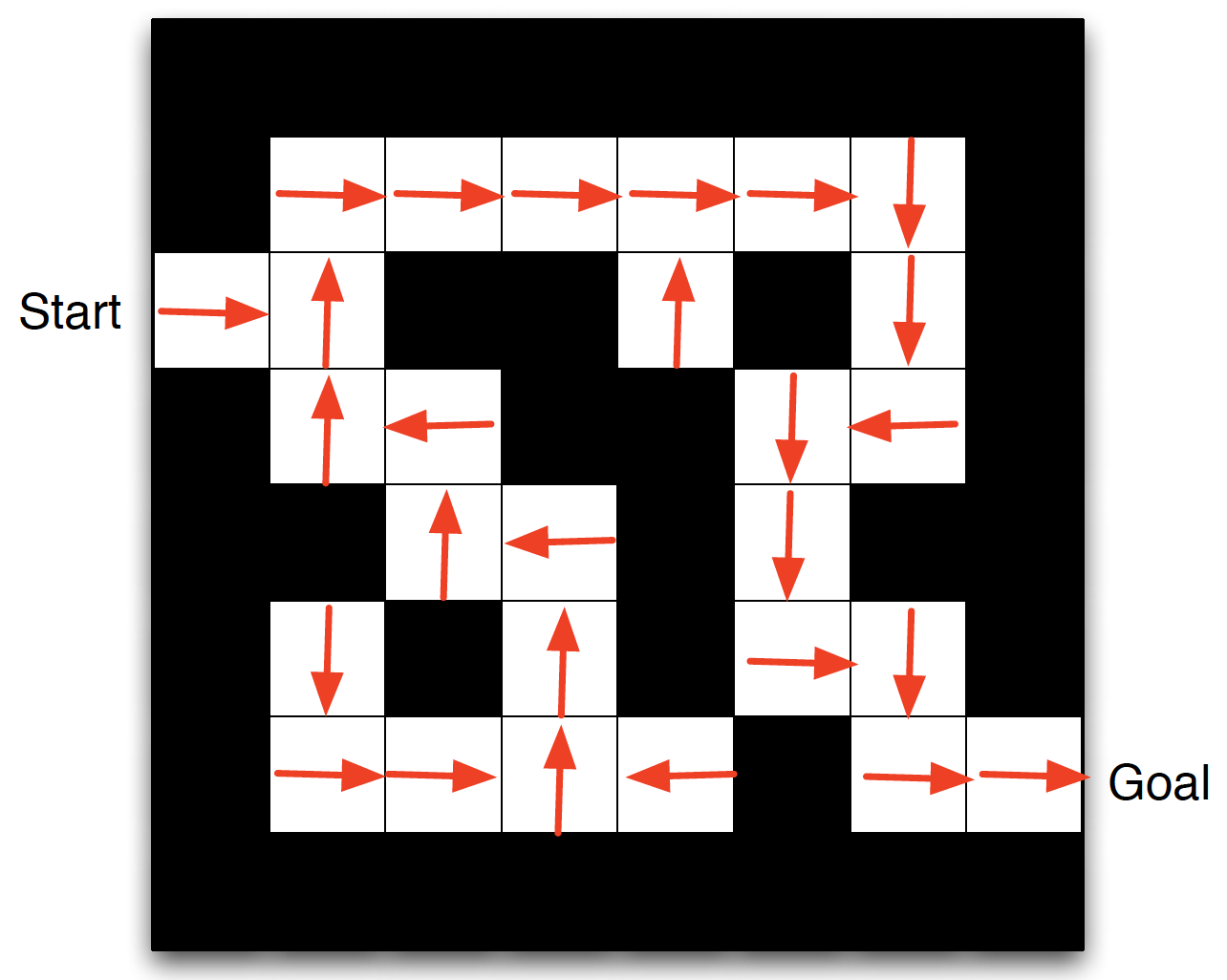
• Policy function: the agent’s behaviour function, the way the agent chooses actions. It can be thought of as the map between state and action. In the maze example, it could be

• Value function: how the agent thinks he is doing. This is a prediction of future rewards.

\[\begin{equation*} v_{\pi}(s) = E\left[R_{t+1} + \gamma R_{t+2} + \gamma^2 R_{t+3} + \cdots |S_t = s\right]. \end{equation*}\]

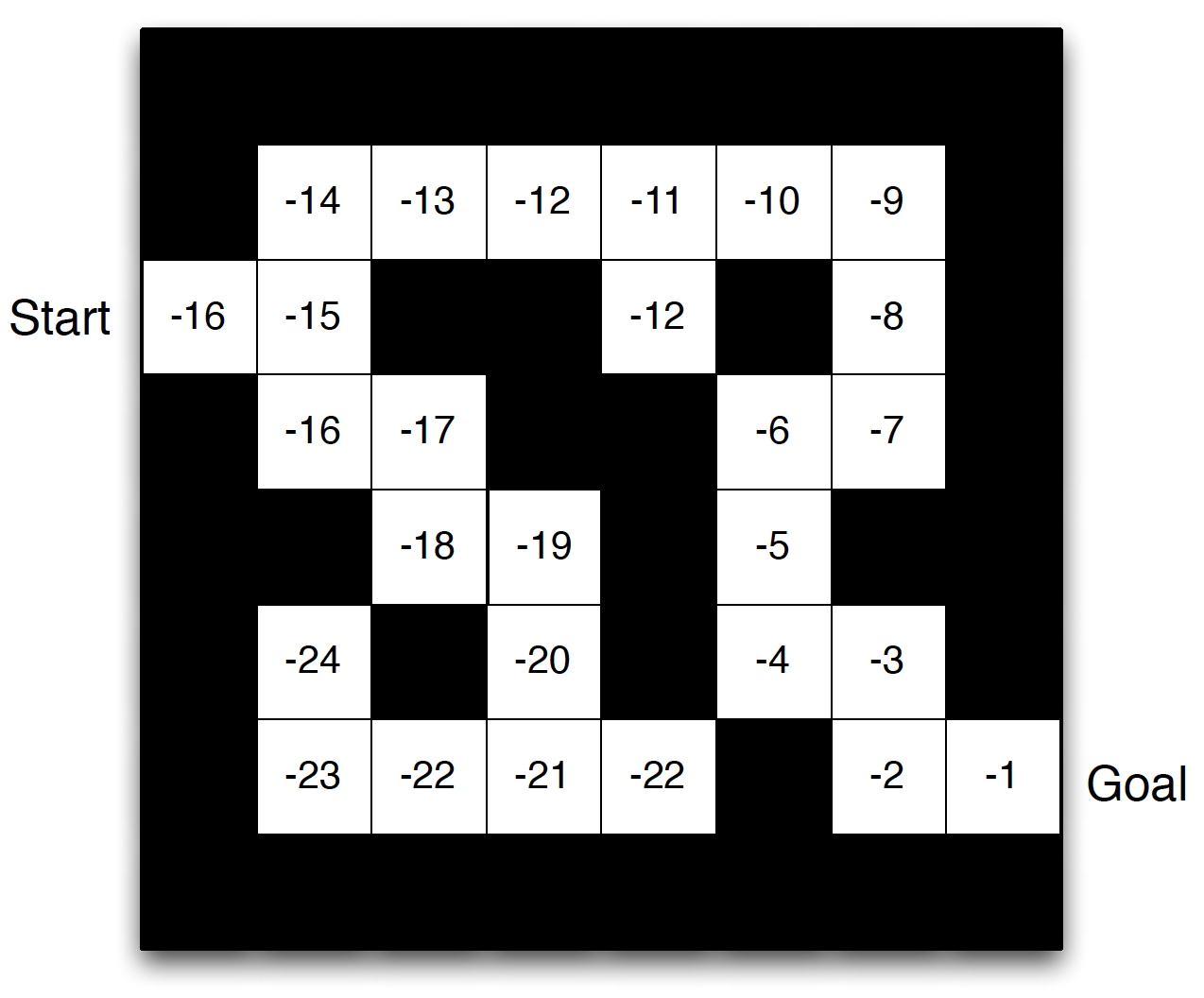
Note that if we have a value function, we do not explicitly require a policy function. This is because we can decide on our actions by choosing an action that leads to the state with the highest value.

• Model: the agent’s representation of the environment. A model predicts what the environment is going to do next. It itself consists of two parts: transitions and rewards. Model is not the environment itself. Note that having a model is not required. Many methods in RL are actually model-free.

The above leads us to the following taxonomy of an RL agent: policy-based vs. value-based. The former one does not require a value function. Instead, he directly works with the policy function. The latter is the opposite. That is, it only requires the value function. An agent that combines policy and value function is know as an “actor critic” agent.

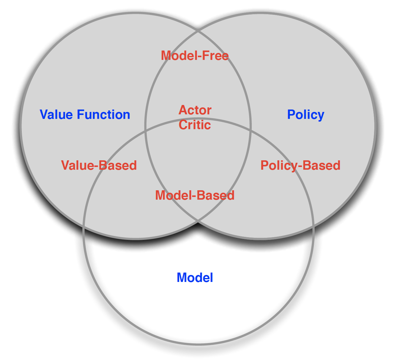
Similarly, with respect to model, we distinguish between model-free and model-based RL agents. Model-free agents only require policy and/or value function. Model-based approaches also require a model of the environment.

Note a difference between the RL problem and the planning problem. The RL problem can be summarized as

• the environment is initially unknown
• the agent interacts with the environment
• the agent improves its policy

Planning, on the other hand, is characterized as

• the model of the environment is known
• the agent performs computations with the model (without any external interactions)
• the agent improves the policy

There is a distinction in RL between prediction and control. The former tries to evaluate the future given a policy. The latter tries to find the best policy. In many cases, we need to first solve the prediction problem to successfully tackle the control problem.

Another central concept to RL is the tradeoff between exploration and exploitation. There should be a balance between how much an agent should explore the environment before he can start to exploit the knowledge he has accumulated.

Markov Processes

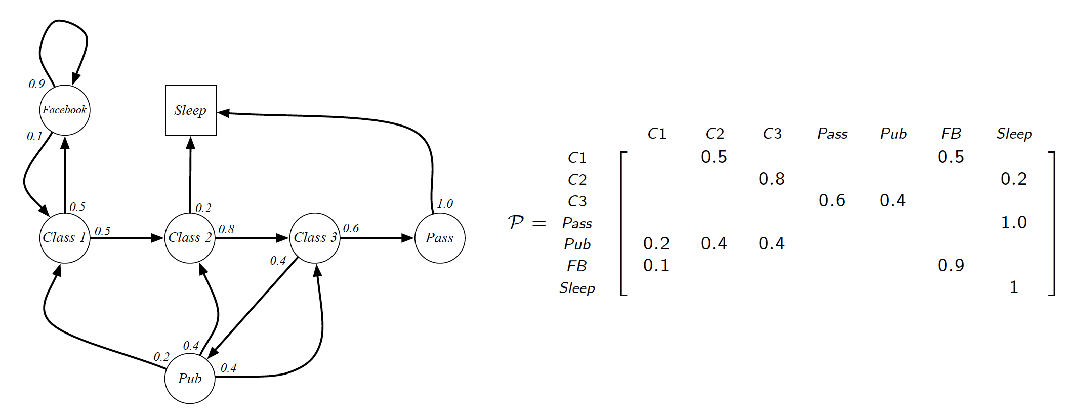
Markov Decision Processes (MDPs) formally describe an environment for RL. Almost any RL problem can be described as an MDP (this applies to partially observable problems as well). For a Markov chain of states $S$, the state transition probabilities are defined as

\[\begin{equation*} P_{ss'} = P\left[S_{t+1}=s'|S_t=s\right]. \end{equation*}\]

These probabilities can be combined into a state transition matrix $P$, where each row sums up to 1.

Markov process is a memoryless process, i.e. a sequence of random states $S_1, S_2,…, S_t$ with the Markov property. A Markov process (Markov chain) is a tuple $<S, P>$, where

• $S$ is a finite set of states,
• $P$ is state transition matrix.

A sample from a Markov process is nothing else but a sequence of visited states. Note that these realization can all be of different lengths, i.e. some realizations may lead to the terminal state before others.

Markov Reward Processes

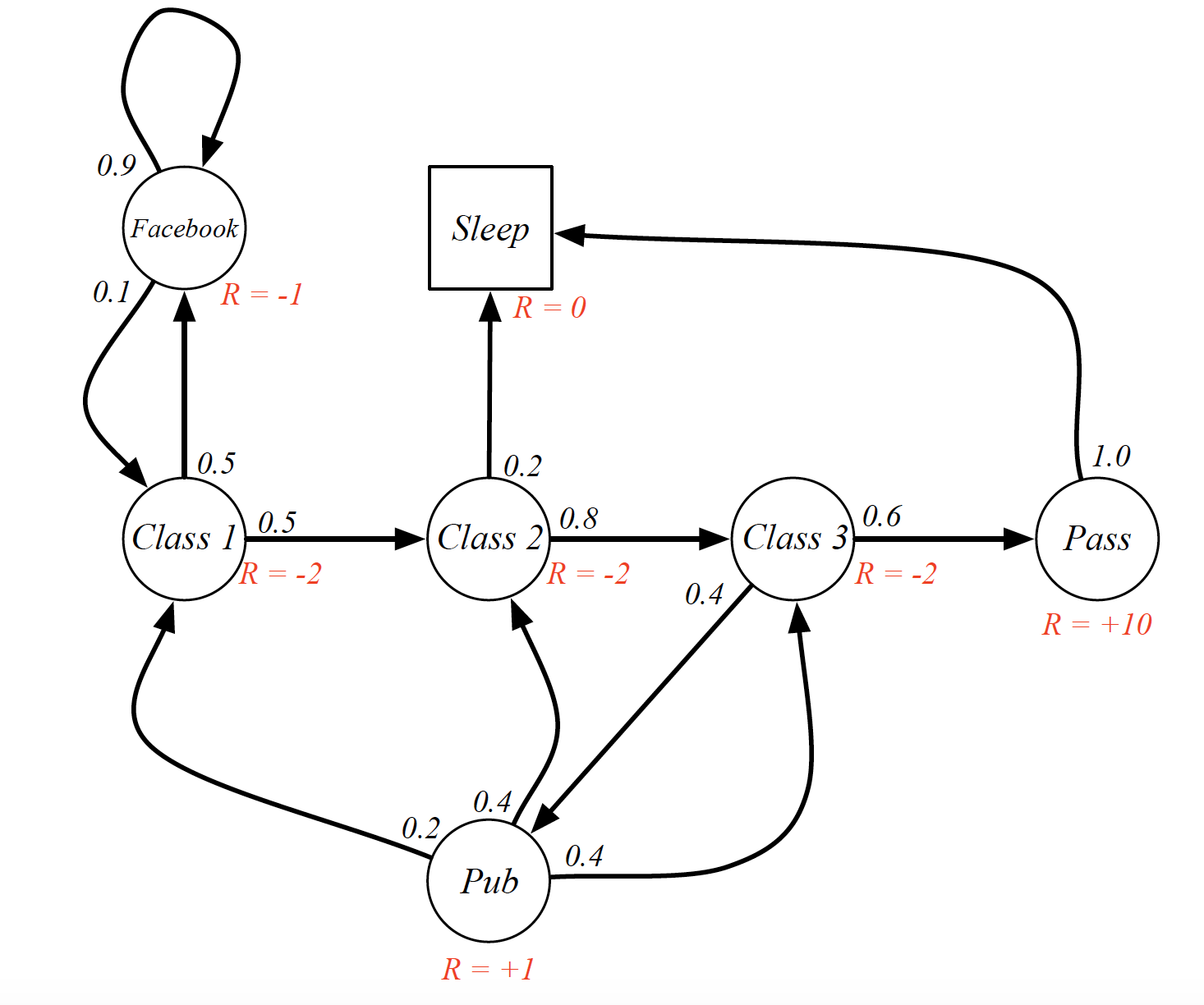
Markov Reward Process (MRP) builds upon simple Markov processes by adding rewards. So, MRP is a tuple $<S, P, R, \gamma>$, where

• $S$ is a finite set of states,
• $P$ is state transition matrix,
• $R$ is a reward function such that

\[\begin{equation*} R_s = E\left[R_{t+1}|S_t=s\right]. \end{equation*}\]

Note that, in practical applications, reward is usually a function of the state. For example, in atari games, reward would be given based on what is going on on the screen.

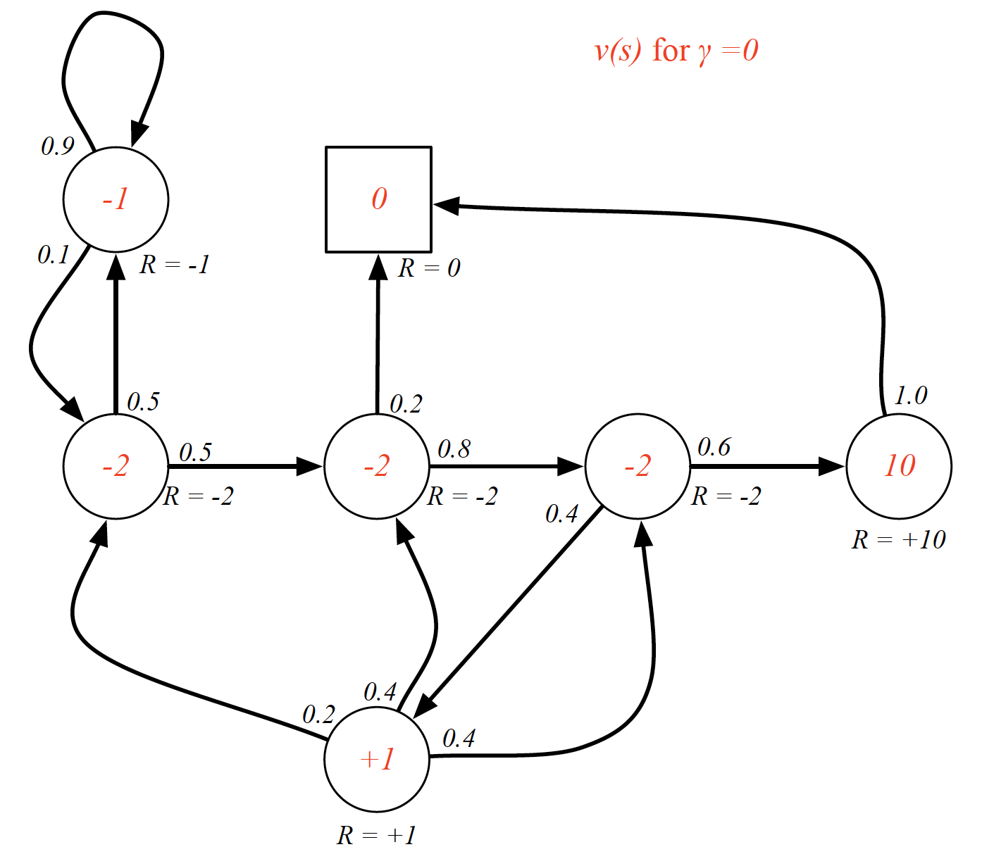
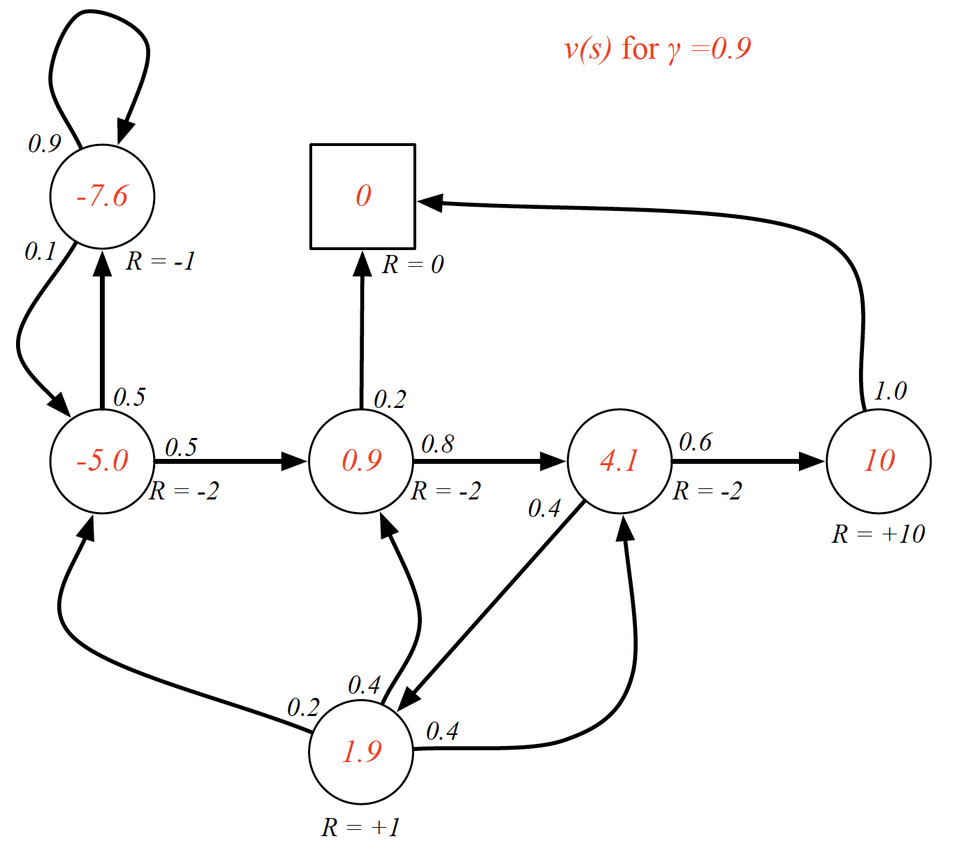
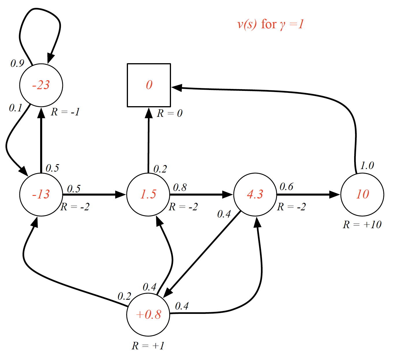
• $\gamma \in [0,1]$ is a discount factor. A value of gamma close to 0 means that we only care about immediate rewards. On the other hand, a value of gamma close to 1 signifies that we care a lot about our future rewards. The reason why we are using a discount factor is to reflect the fact that the future rewards are less certain, i.e. we cannot fully rely on obtaining them. Note that it is possible to use undiscounted Markov reward process, i.e. a value of 1 for $\gamma$, if all the sequences terminate.

The return, $G_t$, is the sum of future discounted rewards from time $t$. That is,

\[\begin{equation*} G_t = R_{t+1} + \gamma R_{t+2} + \gamma^2 R_{t+3} + \cdots \end{equation*}\]

The state value function, $v(s)$, of an MRP is the expected return starting from state $s$, i.e.

\[\begin{equation*} v(s) = E\left[G_t|S_t=s\right]. \end{equation*}\]

It gives a long-term value for each state.

Bellman equation writes the “value” of a decision problem at a certain point in time in terms of the payoff from some initial choices and the “value” of the remaining decision problem that results from those initial choices. Applying the Bellman equation to the value function, we can split it into two parts:

• the expected immediate reward $R_{t+1}$
• the expected discounted value of the next step

In other words,

\[\begin{align*} v(s) &= E\left[R_{t+1} + \gamma R_{t+2} + \gamma^2 R_{t+3} + \cdots |S_t=s\right] \\ &= E\left[R_{t+1} + \gamma \left(R_{t+2} + \gamma R_{t+3} + \cdots\right)|S_t=s\right] \\ &= E\left[R_{t+1} + \gamma E\left[R_{t+2} + R_{t+3} + \cdots|S_{t+1}\right]|S_t=s\right] \\ &= E\left[R_{t+1} + \gamma * v\left(S_{t+1}\right)|S_t =s\right], \end{align*}\]

where we used the fact that $E\left[X\right|G_1] = E\left[E\left[X|G_2\right]|G_1\right]$ if $G_1 \subseteq G_2$.

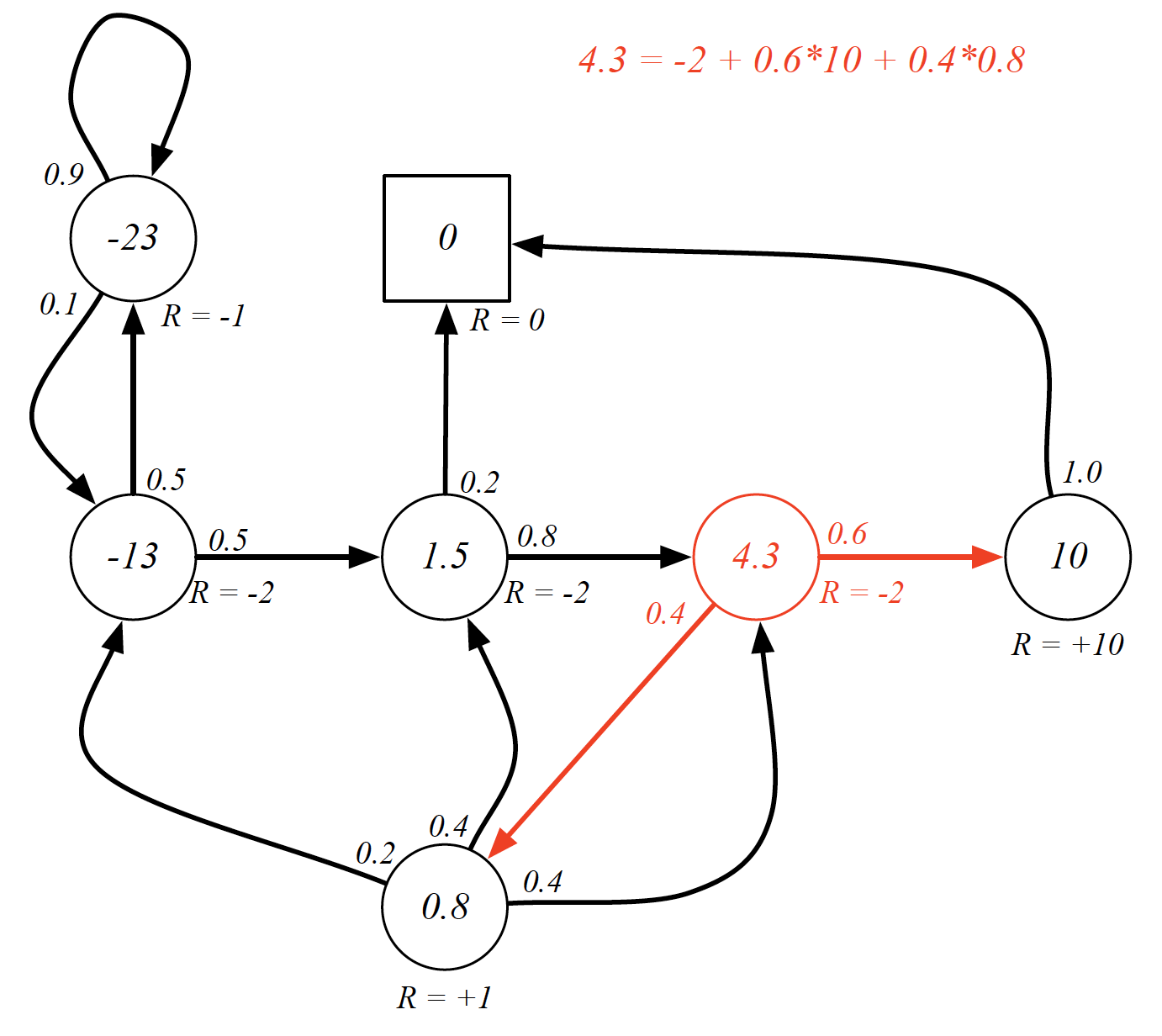
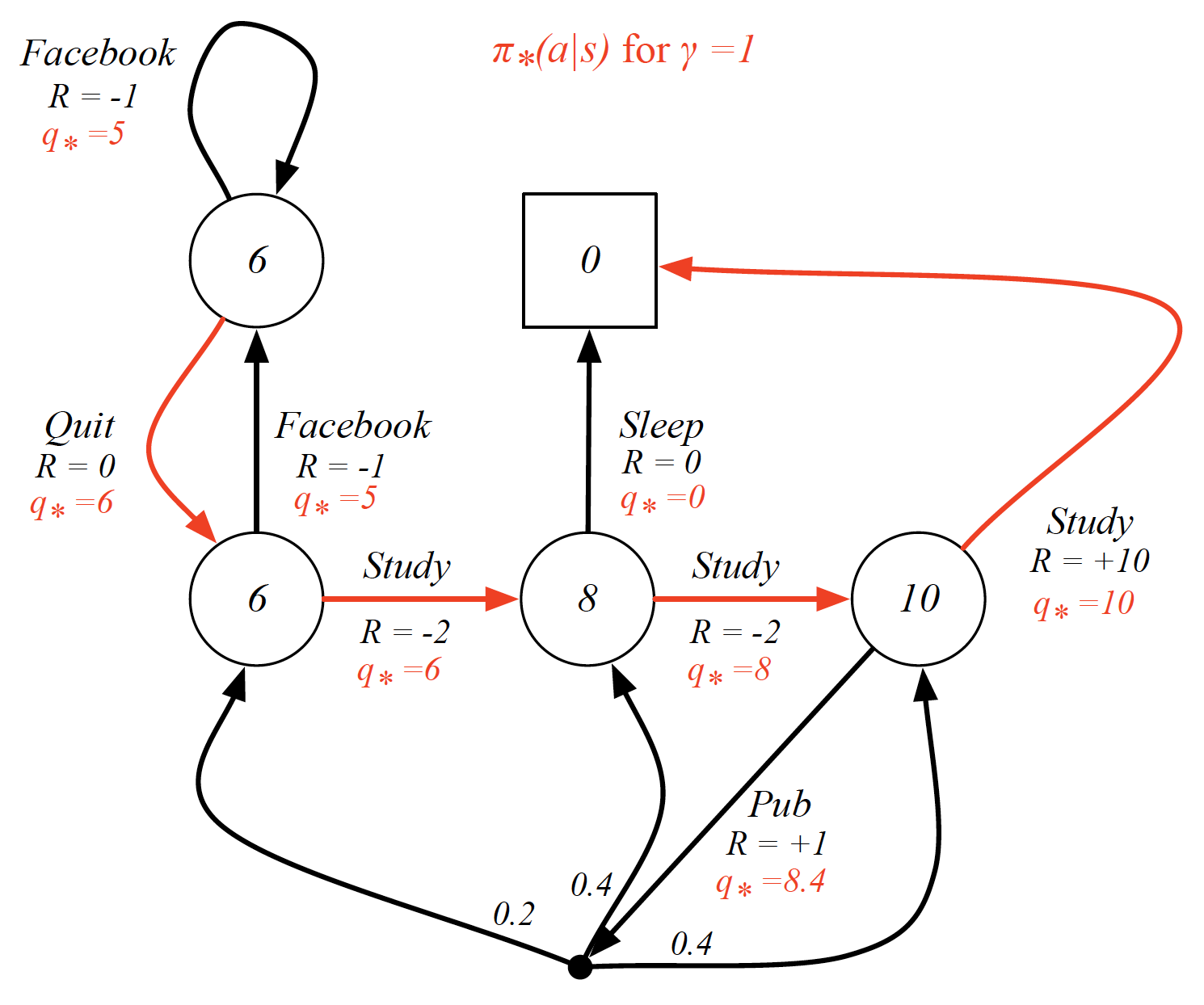
For example,

All the value functions should satisfy the Bellman equation. If they do not, then we did not find the value function. We can represent the Bellman equation in matrix form as follows

\[\begin{equation*} \pmb{v} = R + \gamma P \pmb{v} \end{equation*}\]

where $\pmb{v}$ is a column vector and each row represents the value of each separate state, $R$ is a reward vector associated with each of the states, $P$ is state transition matrix. We can easily find a solution to the above equation as follows:

\[\begin{align} \pmb{v} - \gamma P \pmb{v} &= R \nonumber \\ \left(I - \gamma P\right)\pmb{v} &= R \nonumber \\ \pmb{v} = \left(I - \gamma P\right)^{-1} R. \label{eq:linear_solution} \end{align}\]

In other words, if we know all the reward vector and the state transition matrix, we can find the value of each step directly. However, this way of estimating the value function is only feasible for small MRPs as the complexity is $O(n^3)$. Other methods of solving include:

• dynamic programming
• Monte-Carlo evaluation
• temporal difference

Markov Decision Processes

Markov Decision Process (MDP) is an MRP with actions. So, MDP is a tuple $<S, A, P, R, \gamma>$, where:

• $S$ is a finite state space, each state is Markov
• $A$ is a finite action space
• $P$ is state transition matrix such that

\[\begin{equation*} P_{ss'}^a = P\left[S_{t+1}=s'|S_t=s, A_t=a\right]. \end{equation*}\]

• R is a reward function such that

\[\begin{equation*} R_s^a = E\left[R_{t+1}|S_t=s, A_t=a\right]. \end{equation*}\]

• $\gamma$ is a discount factor

In MDPs we also have a policy, which is the distribution over actions given states. Mathematically,

\[\begin{equation*} \pi\left(a|s\right) = P\left[A_t=a|S_t=s\right]. \end{equation*}\]

The policy fully defines the behaviour of the agent. Note that there is no subscript for time in the equation for policy. This is because we only consider stationary policies, i.e. policies that are not time dependent.

Given an MDP $<S, A, P, R, \gamma>$ and a fixed policy $\pi$, a sequence of states is a Markov chain, i.e. $<S, P^{\pi}>$ is a Markov chain; a sequence of states and rewards is a Markov reward process, i.e. $<S, P^{\pi}, R^{\pi}, \gamma>$ is a an MRP, where

\[\begin{align*} P_{ss'}^{\pi} &= \sum_{a\in A}{\pi(a|s) P_{ss'}^{a}}, \\ R_s^{\pi} &= \sum_{a\in A}{pi(a|s) R_s^a} \end{align*}\]

This basically means that we can recover a Markov chain or an MRP from an MDP. According to Wikipedia, once we have combined an MDP with a policy, we “fixed the action for each state and the resulting combination behaves like a Markov chain”. In other words,

\[\begin{equation*} v_{\pi} = R^{\pi} + \gamma P^{\pi}v_{\pi}, \end{equation*}\]

where $R^{\pi}$ is the averaged (over all actions under policy $\pi$) reward and $P^{\pi}$ is the average state transition matrix. We can solve for the value function by using Equation $\left(\ref{eq:linear_solution}\right)$.

State-value function $v_{\pi}(s)$ of an MDP is the expected sum of future rewards if we start in state $s$ and proceed by following policy $\pi$. In particular,

\[\begin{equation} v_{\pi}(s) = E_{\pi}\left[G_t|S_t=s\right]. \label{eq:state_value_func} \end{equation}\]

Action-value function $q_{\pi}(s, a)$ of an MDP is the expected sum of future rewards if we start is state $s$ and take action $a$. Hence,

\[\begin{equation*} q_{\pi}(s, a) = E_{\pi}\left[G_t|S_t=s, A_t=a\right]. \end{equation*}\]

Since both $v_{\pi}(s)$ and $q_{\pi}(s,a)$ are value functions, each can be decomposed into two components according to the Bellman equation.

The following relationship exists between the state-value function and the action-value function:

\[\begin{equation} v_{\pi}(s) = \sum_{a\in A}\pi\left(a|s\right)q_{\pi}(s,a). \label{eq:simpl} \end{equation}\]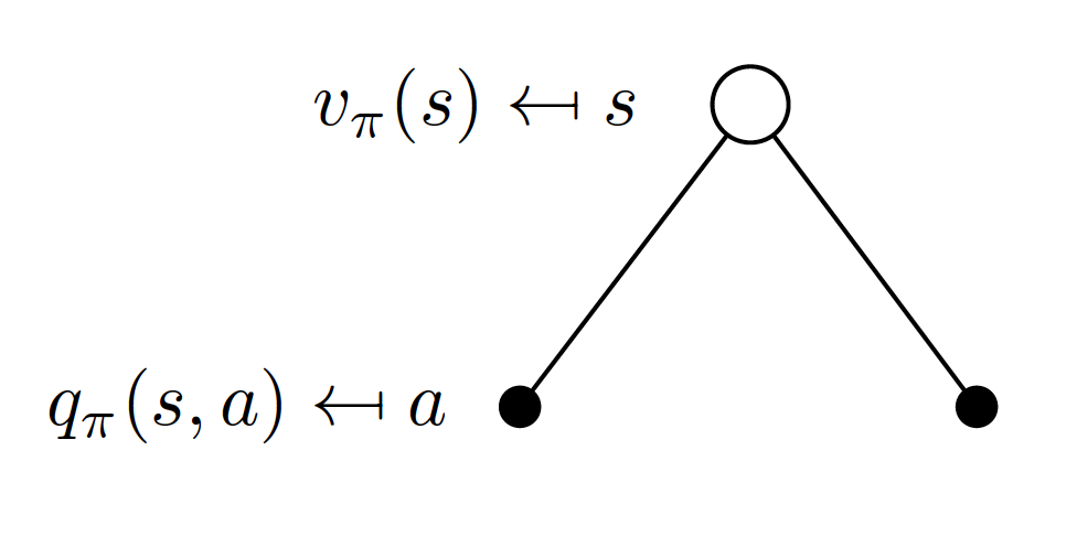

In other words, for a given strategy $\pi$, the value of any state is probability-weighted average of action-state values. In a similar fashion, we can express the relationship between the action-state function and the state-value functions of the following state. What we mean is

\[\begin{equation*} q_{\pi}(s, a) = R_s^a + \gamma\sum_{s'\in S} P_{ss'}^{a}v_{\pi}(s'). \end{equation*}\]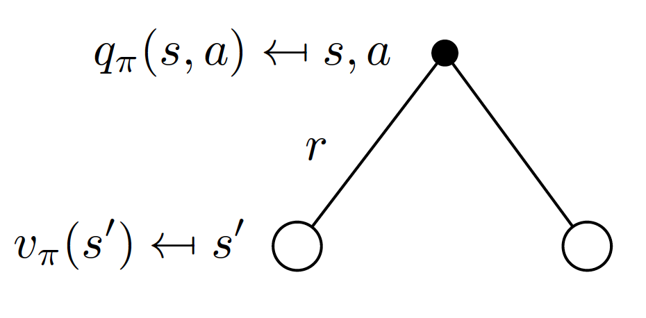

Combining Equations $\left(\ref{eq:state_value_func}\right)$ and $\left(\ref{eq:simpl}\right)$, we get the following representation of state-value function:

\[\begin{equation} v_{\pi}(s) = \sum_{a\in A}\pi\left(a|s\right) \left(R_s^a + \gamma\sum_{s'\in S} P_{ss'}^{a}v_{\pi}(s')\right). \label{eq:representation} \end{equation}\]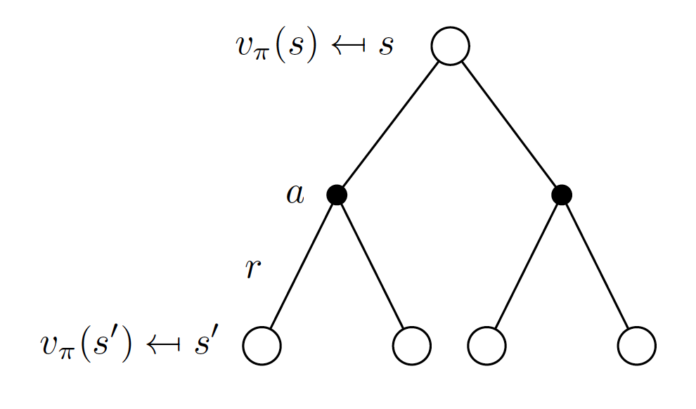

In a similar fashion, we can represent the action-value function $q_{\pi}(a,s)$ as follows:

\[\begin{equation} q_{\pi}(s, a) = R_s^a + \gamma\sum_{s'\in S} P_{ss'}^{a}\sum_{a'\in A}\pi\left(a'|s'\right)q_{\pi}(s',a'). \label{eq:representation2} \end{equation}\]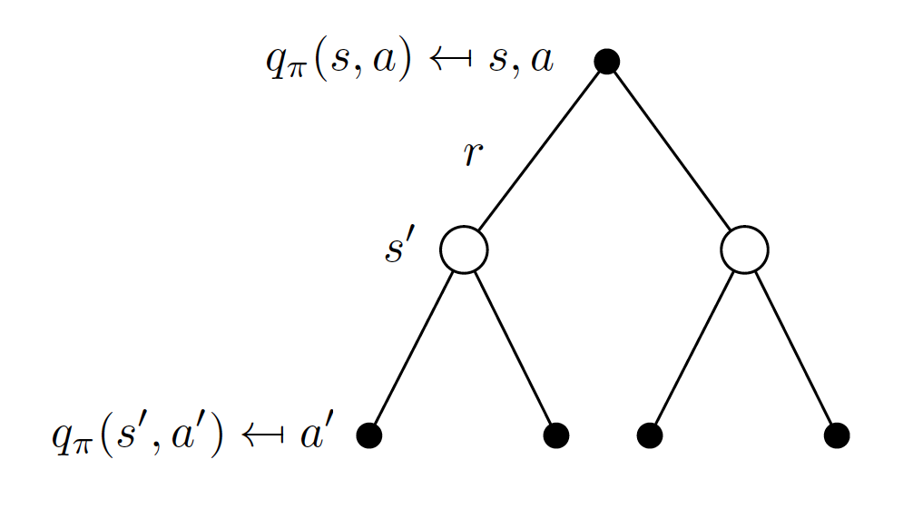

Equations $\left(\ref{eq:representation}\right)$ and $\left(\ref{eq:representation2}\right)$ are known as Bellman expectation equations.

Optimal Value Functions and Policies

To find a solution to an MDP means to find the optimal policy, i.e. the optimal course of action. However, we need to first define what we mean by optimal. The optimal state-value function $v^*(s)$ is defined as

\[\begin{equation*} v^*(s) = \max_{\pi}v_{\pi}(s). \end{equation*}\]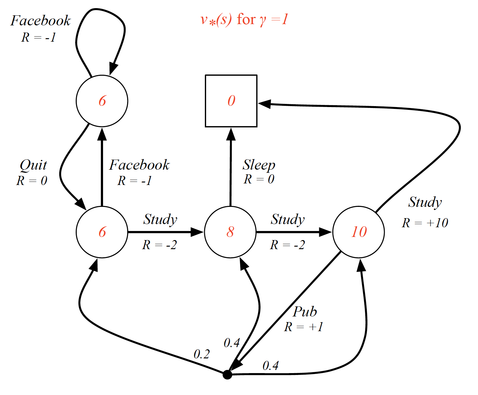

Similarly, the optimal action-state value $q^*(s,a)$ is the one such that

\[\begin{equation*} q^*(s,a) = \max_{\pi}v_{\pi}(s,a). \end{equation*}\]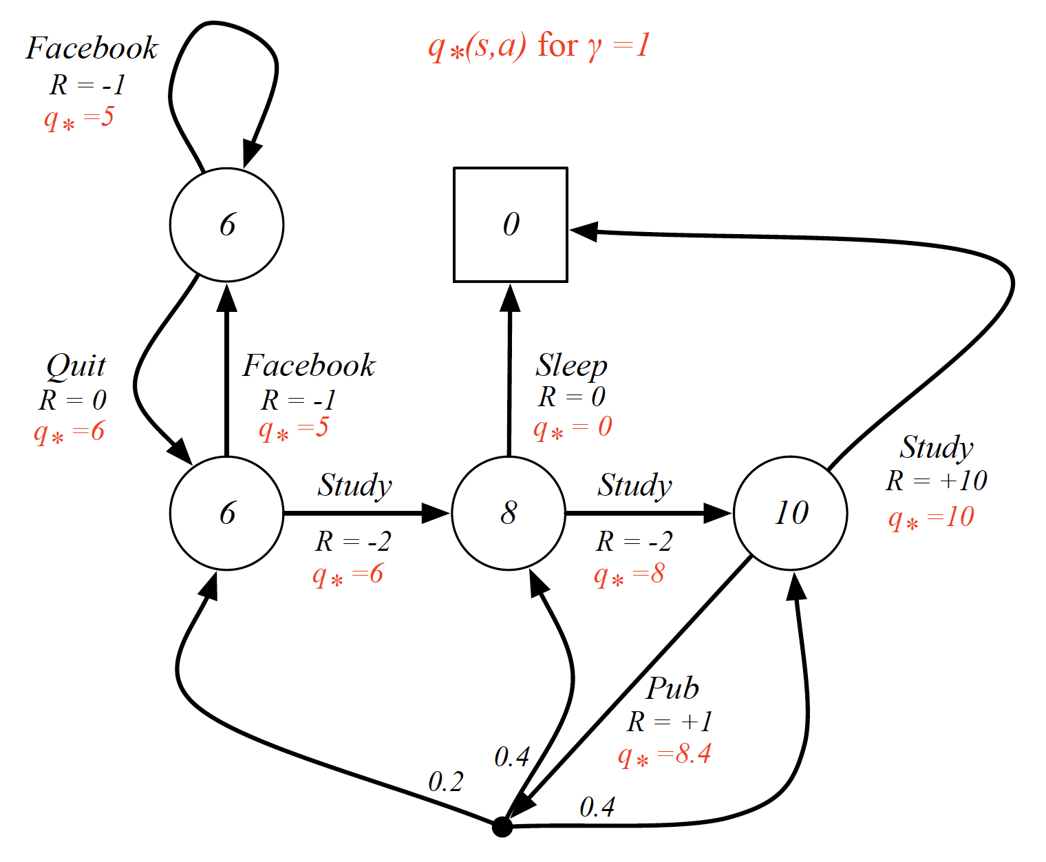

By the way, if we know $q^*(s,a)$, we are basically done, i.e. we know how to behave optimally to optimize our long term behavior. It further means that solving an MDP means solving for the optimal action-state value.

Let us define a partial order of policies as follows

\[\begin{equation*} \pi >= \pi' \hspace{2mm} \text{if} \hspace{2mm} v_{\pi}(s) >= v_{\pi'}(s), \forall s\in S. \end{equation*}\]

The following theorem is very important in the theory of MDPs

• for any MDP, there exists an optimal policy $\pi^*$ that is better than or equal to all other policies $\pi, \forall \pi$
• all optimal policies achieve the optimal state-value function, i.e. $v_{\pi^*}(s)=v^*(s)$
• all optimal policies achieve the optimal actions-value function, i.e. $q_{\pi^*}(s,a)=q^*(s,a)$

An optimal policy is then

\[\begin{equation*} \pi^*(a|s) = \begin{cases} 1, \hspace{2mm} \text{if} \hspace{2mm} a = \underset{a\in A}{argmax} \hspace{2mm}q_{\pi^*}(s,a) \\ 0, \hspace{2mm} \text{otherwise} \end{cases} \end{equation*}\]

It is important to mention now that there is always a deterministic optimal policy for an MDP. In other words, for any kind of MDP, we can find an optimal policy that will assign a probability of 1 to the action with the highest action-value and 0 to all other states.

Finding the Optimal Action-Value Function

So how do we figure out the optimal state-value and action-value functions? Similar to Equation $\left(\ref{eq:simpl}\right)$, we can use use Bellman optimality equations to find the relationships between the optimal state-value functions between states. In particular,

\[\begin{equation*} v^*(s) = \max_{a \in A}q^*(s,a). \end{equation*}\]

Note that we no longer average over different actions (as was the case with Equation $\left(\ref{eq:simpl}\right)$). This is because, under the optimal policy $\pi^*$, we can choose the best action with probability 1 and the value of our state is equal to the optimal action-value.

We express the optimal action-value function in the same way, i.e.

\[\begin{equation*} q^*(s,a) = R_s^a + \gamma \sum_{s' \in S}P_{ss'}^a v^*(s'). \end{equation*}\]

In other words the value taking any action $a$ in any state $s$ is equal to the immediate reward plus the expected state values of the next states.

Combining the two together, we get

\[\begin{equation} v^*(s) = \max_{a \in A} \left(R_s^a + \gamma \sum_{s' \in S}P_{ss'}^a v^*(s')\right). \label{eq:optimal_state_value_func} \end{equation}\]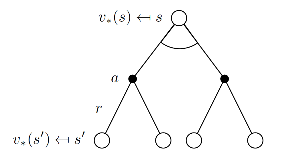

Similarly, we can express the optional action-value function as

\[\begin{equation} q^*(s,a) = R_s^a + \gamma \sum_{s' \in S}P_{ss'}^a \max_{a' \in A}q^*(s', a'). \label{eq:optimal_action_value_func} \end{equation}\]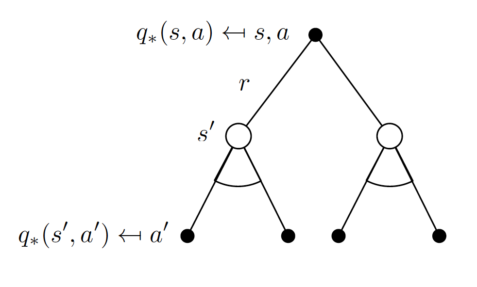

Equations $\left(\ref{eq:optimal_state_value_func}\right)$ and $\left(\ref{eq:optimal_action_value_func}\right)$ are known as Bellman optimality equations. They tell us how the optimal state-value and action-value functions in state $s$ are related to the optimal state-value and action-value functions of the subsequent states and actions.

These Bellman optimality equations are not linear. Thus, iterative approaches are needed:

• value iteration
• policy iteration
• Q-learning
• SARSA

Planning by Dynamic Programming

Dynamic programming is used whenever we can break down a problem into smaller components. We say that a problem has optimal substructure if the problem can be solved optimally by breaking it into sub-problems and then recursively finding the optimal solutions to the sub-problems. If sub-problems can be nested recursively inside larger problems, so that dynamic programming methods are applicable, then there is a relation between the value of the larger problem and the values of the sub-problems. In the optimization literature this relationship is called the Bellman equation.

As we already know, we can express the relationships between state-value and action-value functions of MDPs via Bellman equations. In particular, Bellman equations give us recursive decompositions, i.e. to behave optimally in the long-run, we need to behave optimally for a single time step and then continue behaving optimally for all other time steps. Furthermore, value functions store and reuse the estimated values. This means that if we have already figured out the state-value or action-value functions for states close to the terminal step, we do not need to recalculate them again. Instead, we can start working backwards to solve for state-value and action-value functions of the preceding states. Hence, dynamic programming techniques are applicable to MDPs.

Using DP requires full knowledge of the MPD, i.e. we need to know all the states, state transition matrix, rewards for each state, all possible actions and the discount factor. It further means that we must know everything about the environment. Thus, it is not really an RL problem. DP is used for planning in an MDP:

• Prediction or Policy Evaluation
  We are given an MDP $<S, A, P, R, \gamma>$ and policy $\pi$ as input. We need to find the value function $v_{\pi}$ associated with the policy.
• Control
  We are given an MDP $<S, A, P, R, \gamma>$ as input. We need to find out the optimal value function $v^*$ from which the optimal policy $\pi^*$ follows.

Policy Evaluation

In this problem, we want to estimate the value function for an MDP $<S, A, P, R, \gamma>$ given some policy $\pi$. One way to solve the problem is to iteratively apply the Bellman expectation backup. The algorithm works in the following way:

• randomly initialize the values for the state-value function $v$. Let the starting point be $\pmb{v}_0$ (a vector of state-values for all $s \in S$).
• for each iteration i, update $v_i(s)$ using the Bellman expectation equations and using the values from the previous iteration $v_{i-1}(s’)$, where $s’$ is the successor state to state $s$.

In other words, we are using the state values of the successor states of the previous iteration to update the state value of the root of the current iteration. This algorithm is known as synchronous backup because we are updating the value function for all the states simultaneously. The actual update formula is as follows

\[\begin{align} v_{i}(s) = \sum_{a \in A} \pi(a|s) \left(R_s^a + \gamma \sum_{s' \in S}P_{ss'}^a v_{i-1}(s')\right). \label{eq:policy_evaluation} \end{align}\]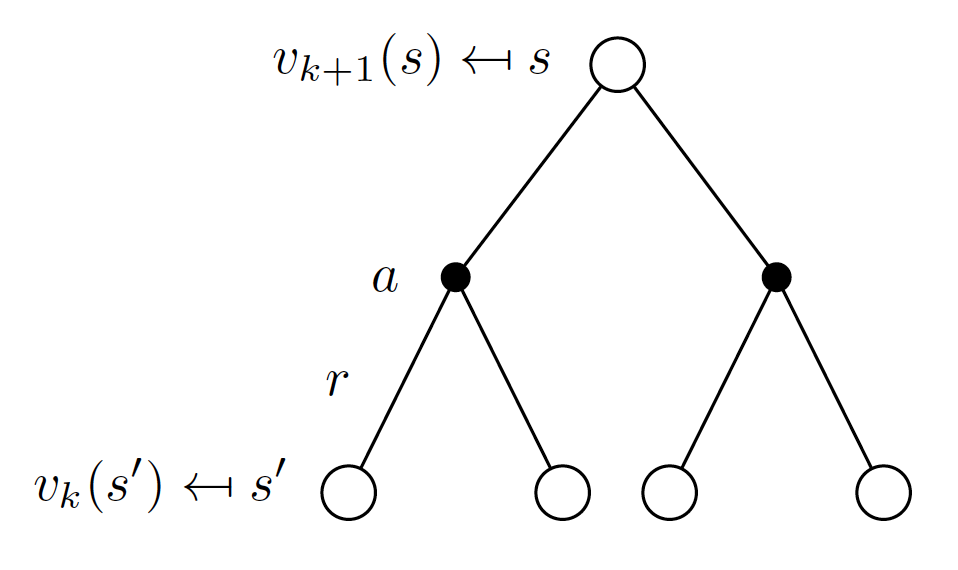

In matrix form:

\[\begin{equation*} \pmb{v}_{i} = R^{\pi} + \gamma P^{\pi}\pmb{v}_{i-1}. \end{equation*}\]

This procedure is guaranteed to converge to the true state-value function of the MDP.

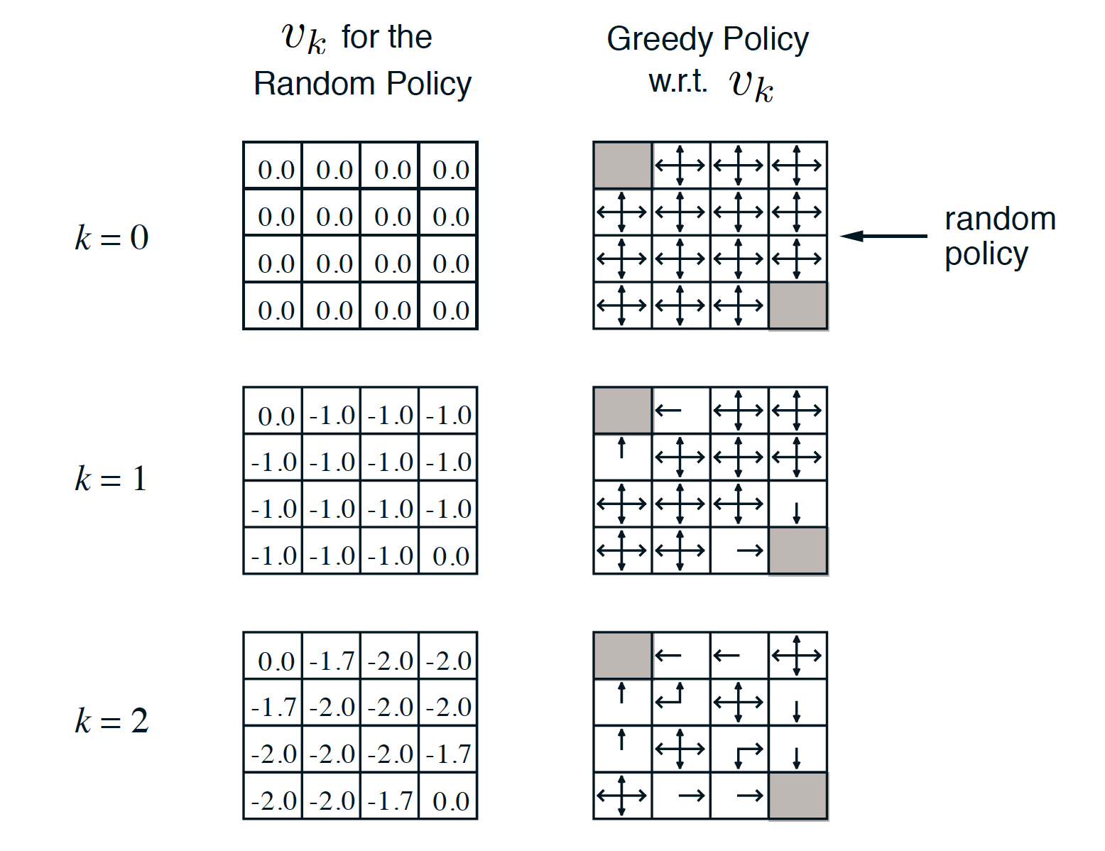
Example

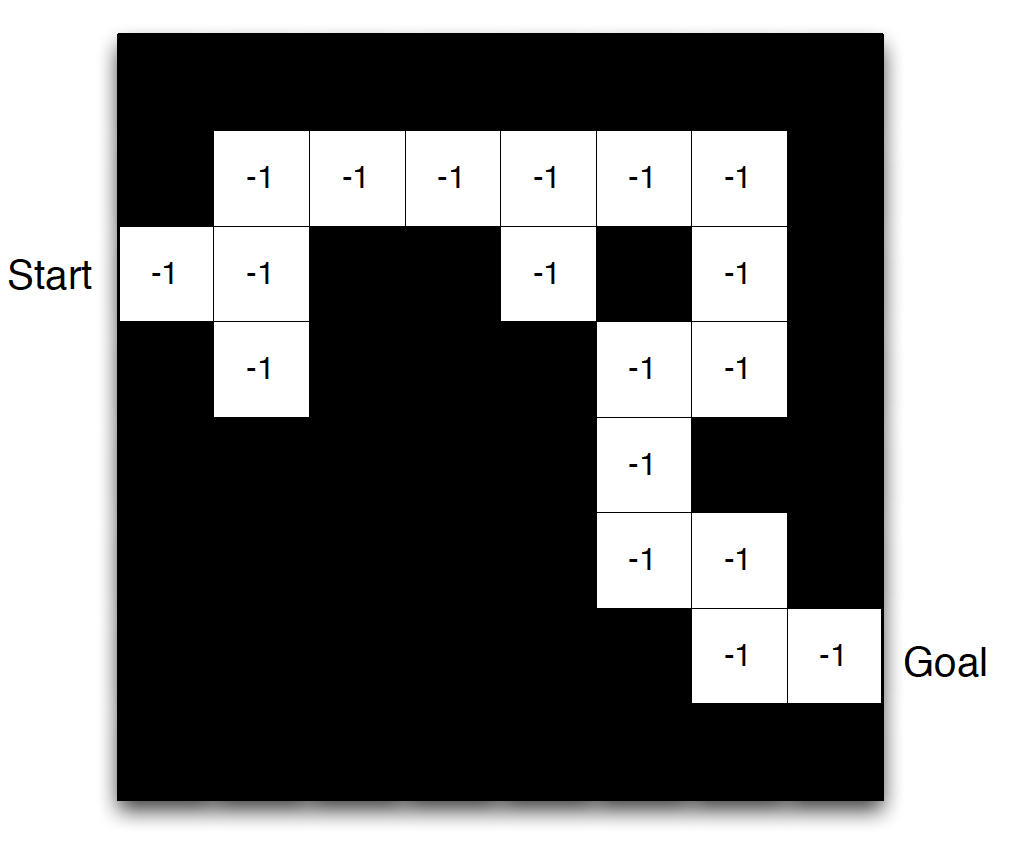
Consider the following environment:

\[\begin{equation*} S = \left[ \begin{matrix} s_{T} & s_{12} & s_{13} & s_{14} \\ s_{21} & s_{22} & s_{23} & s_{24} \\ s_{31} & s_{32} & s_{33} & s_{34} \\ s_{41} & s_{42} & s_{43} & s_{T} \end{matrix} \right], \end{equation*}\]

where $s_{T}$ are the two terminal states. Consider the following reward function:

\[\begin{equation*} R = \left[ \begin{matrix} 0 & -1 & -1 & -1 \\ -1 & -1 & -1 & -1 \\ -1 & -1 & -1 & -1 \\ -1 & -1 & -1 & 0 \end{matrix} \right], \end{equation*}\]

i.e. we get $-1$ points for each time step unless we are in the terminal state. We further assume that the discount factor $\gamma$ is equal to $1$.

Out aim is to evaluate a random policy, the policy where the agent can go in any of the four directions: up, down, left or right, with the same probability of $25\%$ (if the agent performs an action that is supposed to take him off the environment, he remains in the same state). Let us initialize our state-value function as follows

\[\begin{equation*} v_{0} = \left[ \begin{matrix} 0 & 0 & 0 & 0 \\ 0 & 0 & 0 & 0 \\ 0 & 0 & 0 & 0 \\ 0 & 0 & 0 & 0 \end{matrix} \right]. \end{equation*}\]

Let us perform the first iteration of state-value function update.

\[\begin{equation*} v_{1} = \left[ \begin{matrix} 0 & -1 & -1 & -1 \\ -1 & -1 & -1 & -1 \\ -1 & -1 & -1 & -1 \\ -1 & -1 & -1 & 0 \end{matrix} \right]. \end{equation*}\]

Since there is a single action that can be taken in any of the two terminal states (that is, to remain in the terminal state), for the two terminal states we had the following update

\[\begin{align*} v_{1}(s_{T}) &= R_{s_{T}} \\ &= 0. \end{align*}\]

Let consider the state-value update for $s_{12}$.

\[\begin{align*} v_{1}(s_{12}) = \sum_{a \in A}\pi(a|s_{12})\left(R_{s_{12}}^a + \gamma \sum_{s' \in \{s_{T}, s_{12}, s_{13}, s_{22}\}}P_{ss'}^a v_{0}(s')\right). \end{align*}\]

To evaluate the above, we note that

• we can take any of the four actions in state $s_{12}$ with probability $25\%$, i.e. we can go left to end up in the terminal state, go up to remain in the same state, go left to end up in state $s_{13}$ or go down to appear in state $s_{22}$.
• whatever action the agent happens to take, we will receive an immediate reward of $-1$.
• $P_{ss’}^a$ is equal to $1$ for $s’ \in {s_{T}, s_{12}, s_{13}, s_{22}}$ and $0$ otherwise.
• the values of the possible states are taken from $v_0$.
• $\gamma$ is assumed to be equal to $1$.

Thus, we obtain

\[\begin{equation*} v_{1}(s_{12}) = 0.25 \times \left(-1 + 1\times 0\right) + 0.25 \times \left(-1 + 1\times 0\right) + 0.25 \times \left(-1 + 1\times 0\right) + 0.25 \times \left(-1 + 1\times 0\right). \end{equation*}\]

Performing the next iteration of state-value update, we obtain

\[\begin{equation*} v_{2} = \left[ \begin{matrix} 0 & -1.75 & -2 & -2 \\ -1.75 & -2 & -2 & -2 \\ -2 & -2 & -2 & -1.75 \\ -2 & -2 & -1.75 & 0 \end{matrix} \right]. \end{equation*}\]

Let us show how we obtained a value of $-1.75$ for state $s_{12}$.

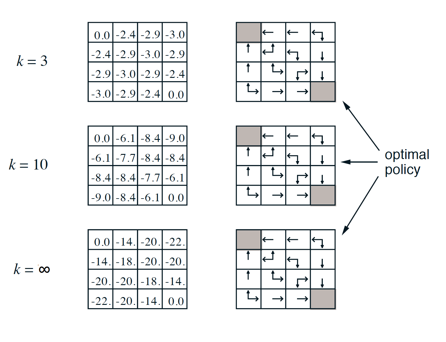
\[\begin{align*} v_2(s_{12}) &= 0.25 \times (-1 - 1 \times 0) + 0.25 \times (-1 - 1 \times 1) + 0.25 \times (-1 - 1 \times 1) + 0.25 \times (-1 - 1 \times 1) \\ &= -1.75 \end{align*}\]

If we continue the iteration algorithm, we will eventually get the true state-value function of the random policy.

\[\begin{equation*} v_{\pi} = \left[ \begin{matrix} 0 & -14 & -20 & -22 \\ -14 & -18 & -20 & -20 \\ -20 & -20 & -18 & -14 \\ -22 & -20 & -14 & 0 \end{matrix} \right], \end{equation*}\]

where each value states how many steps on average it would take an agent who navigates the environment randomly (e.g. random walk) to get to one of the two terminal states.

Policy Iteration

In the policy iteration problem, given an MDP, we want to find the optimal policy $\pi^*$. The procedure is very similar to the one of the previous section but consists of two steps. For each iteration $i$ we do:

• update the state-value function $v_{i}$ under the current policy $\pi_{i-1}$ using the policy evaluation algorithm
• update the policy based on the updated state-value function $v_{i}$, i.e. start acting greedily wrt to $v_{i}$:

\[\begin{equation*} \pi_i = greedy(v_i) \end{equation*}\]

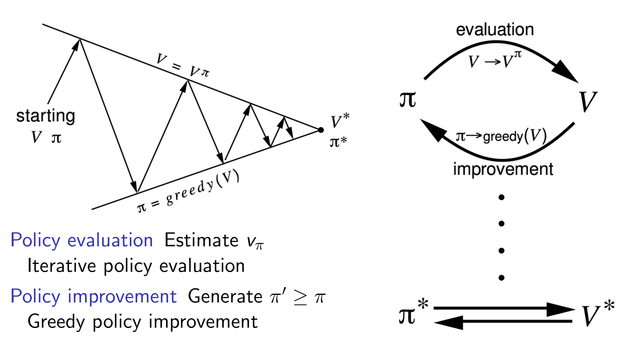
In the long-run, it is guaranteed that our policy will converge to the optimal policy $\pi^*$ regardless of what the initial estimates for the policy / state-value function are taken to be.

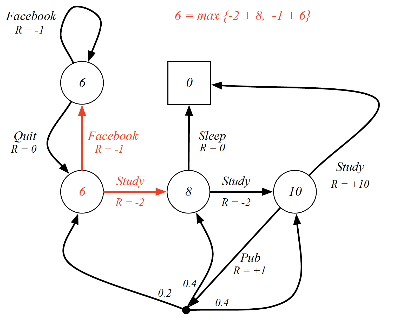
With respect to our previous example, we have

Note that, in the above example, we already obtained the optimal policy after three iterations (even though we do not have the correct/final state-value function).

How do we know what this approach does indeed improve our policy? Put differently, why does the second step of our algorithm, that is starting to act greedily with respect to the updated state-value function, is improving our policy? Let us consider what happens over a single time step. Suppose that our current strategy is deterministic, i.e. $\pi(s)=a$. In other words, for any state $s$, our current policy is to choose some action $a$ with 100% certainty. Taking a greedy action in state $s$ means choosing such action $a$ that maximizes our action-value function in this state, i.e.

\[\begin{equation*} \pi^{'}(s) = \underset{a\in A}{argmax}q_{\pi}(s,a). \end{equation*}\]

The following holds true then

\[\begin{equation} q_{\pi}\left(s, \pi^{'}(s)\right) = \max_{a \in A}q_{\pi}(s,a) \ge q_{\pi}\left(s,\pi(s)\right) = v_{\pi}(s). \label{eq:single_step_greedily} \end{equation}\]

The above equation basically states that taking the greedy action in state $s$ and then returning to policy $\pi$ is at least as good as taking an action $a$ under policy $\pi$ and then following policy $\pi$.

We showed that acting greedily over a single step and getting back to the original policy is at least as good as always acting according to the original policy. Let us now show that acting greedily over all the steps is at least as good as following the original policy. From Equation $\left(\ref{eq:single_step_greedily}\right)$, we get

\[\begin{align*} v_{\pi}(s) &\le q_{\pi}\left(s, \pi^{'}(s)\right) \\ &= E_{\pi}\left[G_t|S_t=s, A_t=\pi^{'}(s)\right] \\ &= E_{\pi}\left[R_{t+1} + \gamma R_{t+2} + \cdots | S_t=s,A_t=\pi^{'}(s)\right] \\ &= E_{\pi^{'}}\left[R_{t+1} + E_{\pi}\left[\gamma R_{t+2} + \gamma^2 R_{t+3} + \cdots |S_{t+1}\right]|S_t=s\right] \\ &= E_{\pi^{'}}\left[R_{t+1} + \gamma v_{\pi}\left(S_{t+1}\right)|S_t=s\right] \\ &\le E_{\pi^{'}}\left[R_{t+1} + \gamma q_{\pi}\left(S_{t+1}, \pi^{'}\left(S_{t+1}\right)\right)|S_t=s\right] \\ &\le E_{\pi^{'}}\left[R_{t+1} + \gamma R_{t+2} + \gamma^2 q_{\pi}\left(S_{t+2}, \pi^{'}\left(S_{t+2}\right)\right)|S_t=s\right] \\ &\le E_{\pi^{'}}\left[R_{t+1} + \gamma R_{t+2} + \gamma^2 R_{t+3} + \cdots | S_t=s\right] \\ &= v_{\pi^{'}}(s). \end{align*}\]

The above tells us that, by following the greedy policy over the whole trajectory, we can expect to get at least as much reward as if we followed the original policy over the whole trajectory.

What happens if there are no more improvements to be made? In other words, what if $q_{\pi}\left(s, \pi^{‘}(s)\right) = \max_{a \in A}q_{\pi}(s,a) = q_{\pi}\left(s,\pi(s)\right) = v_{\pi}(s)$? The answer is: since $v_{\pi}(s)=\max_{a \in A}q_{\pi}(s,a)$, the Bellman optimality equation is satisfied and $v_{\pi}(s) = v^*(s)$ is our optimal policy. Note that the improvement process only ever stops if the optimality equation has been reached.

Value Iteration

What does it mean to follow an optimal policy? The Bellman optimality equation states that following an optimal policy means taking an optimal first step and then following the optimal policy for the remaining trajectory. This means that if we know all the optimal state values of the successor states, we can just find an optimal action over a single step and be done. We have the following theorem:

Theorem (Principle of Optimality): a policy $\pi(a|s)$ achieves the optimal value from state $s, v_{\pi}(s)=v^{*}(s)$, iff, for any state $s’$ reachable from $s$, $\pi$ achieves the optimal value from state $s’, v_{\pi}(s’)=v^{*}(s’)$.

Suppose that we know the values $v^*(s’), \forall s’ \in S$. Using the Bellman optimality equation, we can update the state-value function as follows

\[\begin{equation} v^*(s) \leftarrow \max_{a \in A} \left(R_s^a + \gamma \sum_{s'\in S}P_{ss'}^av^*(s')\right). \label{eq:value_iteration_eq} \end{equation}\]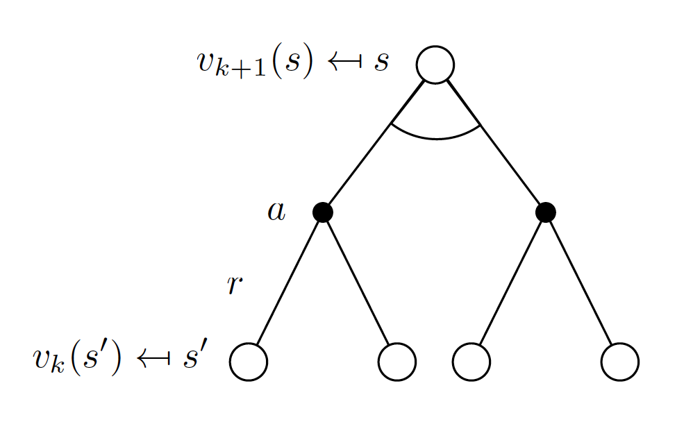

The idea of value iteration is to work backwards by applying updates as per Equation $\left(\ref{eq:value_iteration_eq}\right)$ iteratively.

The problem that value iteration method aims to solve is to find an optimal policy by iteratively applying the Bellman optimality equation. To do that, we perform synchronous backups, i.e. for each iteration $i$ and for all states $s \in S$, update $v_{k+1}(s)$ from $v_k(s)$. Similar to value iteration, we are updating state-value function. However, we are not doing it for any particular policy. Similar to policy iteration, we are trying to find an optimal policy. However, we do not require an explicit policy. Instead, we are directly updating the state-value function. Note that the intermediate state-value function may not correspond to any meaningful or achievable policy.

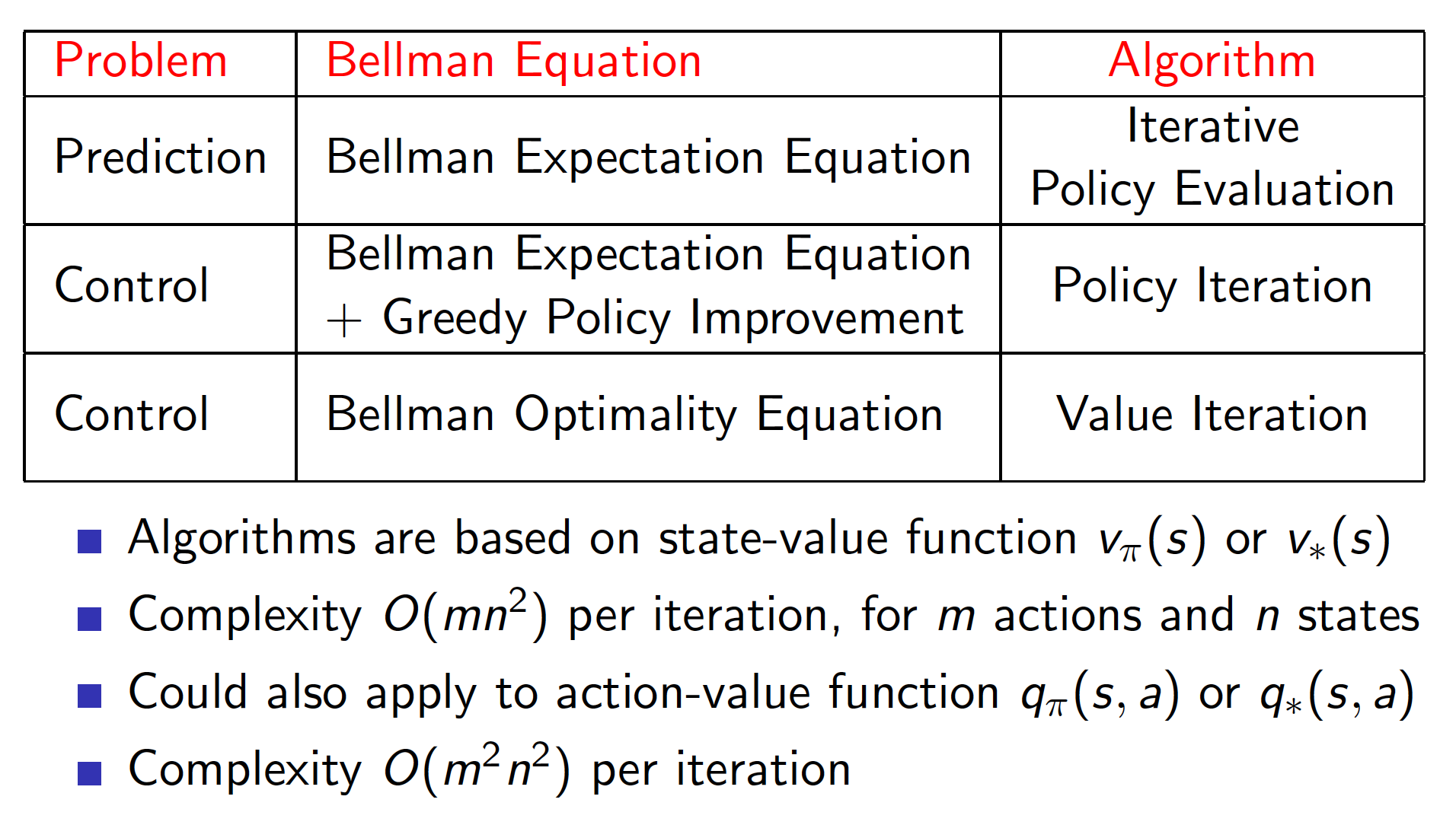
Summary for Synchronous DP Algorithms

Below is the summary of the algorithms that can be used for planning in an MPD.

Asynchronous Dynamic Programming

The algorithms covered up to now update the state-value function for all the states at the same time. However, this is costly if the number of states is too large. For that reason, there are extensions to the synchronous DP algorithms. In particular, we could be smart about which states and in what order to do the state-value update per iteration. The following three approaches are common in practice:

• In-place dynamic programming
  The synchronous state-value update, as in Equation $\left(\ref{eq:policy_evaluation}\right)$ or $\left(\ref{eq:value_iteration_eq}\right)$, requires that we store both the old and the new state values, i.e. from different iterations. In-place dynamic programming, on the other hand, requires that we store a single copy. In other words, for all $s \in S$,

\[\begin{equation*} v(s) \leftarrow \sum_{a \in A}\pi(a|s)\left(R_s^a + \gamma \sum_{s' \in S}P_{ss'}^av(s')\right). \end{equation*}\]

Note that we still update all the states.

• Prioritized Sweeping
  The idea here is to update the states in the order of their significance. For example, we could update the states with the largest remaining Bellman error first, where the remaining Bellman error is

\[\begin{equation*} \left|max_{a \in A}\left(R_s^a + \gamma \sum_{s' \in S}P_{ss'}^av(s')\right) - v(s)\right| \end{equation*}\]

• Real-Time Dynamic Programming
  The idea of real-time DP is to update only those states that are relevant to our agent. For example, if our agent is actively exploring a certain area on the map, it makes little sense to update the states which he has not visited yet. Thus, after each time step $S_t, A_t, R_{t+1}$, update the state $S_t$.

Full-Width Backups

In the DP algorithms we have considered, we used full-width backups (updates). What it means is that to update the value of a given state $s$, we had to look into all the available actions and all the successor states $s’$. Such an approach requires the full knowledge of the MPD, i.e. the reward function and the state-transition function. The full-width backup approach works fine for middle-sized problems. However, as the number of states increases, DP algorithms start to suffer from the curse of dimensionality. More advanced approaches (to be considered later) make the state-value updates by using sample backups, i.e. by using sample rewards and sample transitions $<S, A, R, S’>$.

There are a number of associated advantages:

• Model-free: no need to know the MDP
• Sampling helps to deal with the curse of dimensionality
• The cost of updates are kept constant

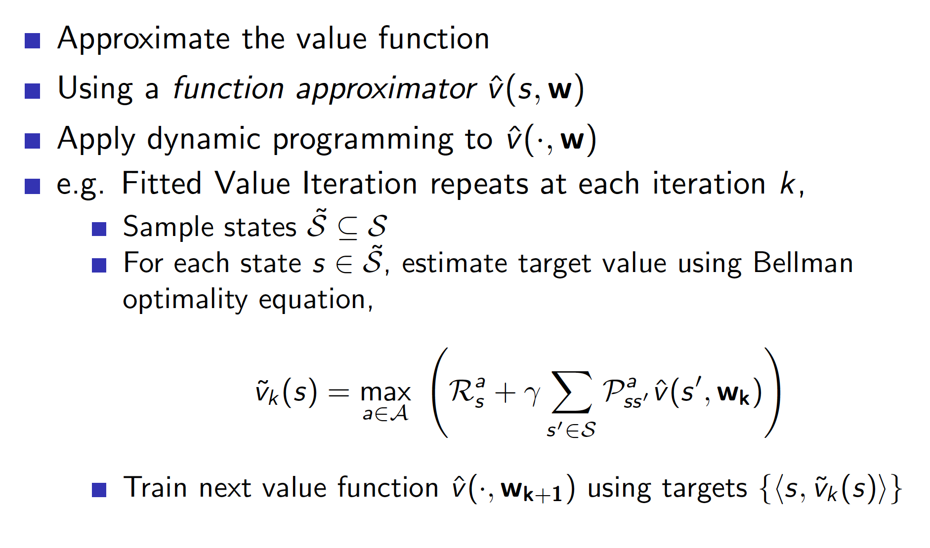
Approximate Dynamic Programming

Model-Free Prediction

We need to use model-free approaches when our agent operates in an environment that can be represented as an MDP but we do not have the knowledge of the MDP. In other words, we do not know the reward function and the state-transition matrix. However, we still want to solve it, i.e. to find an optimal policy. The main methods of model-free prediction are:

• Monte-Carlo Learning
• Temporal Difference (TD) Learning

Note that the problem of prediction is the problem of estimating the value function of an unknown MDP given some policy; the problem of control is the problem of finding a value function corresponding to an optimal policy.

Monte-Carlo Reinforcement Learning

The first model-free method is Monte-Carlo learning. Remember that the aim of prediction is to obtain the state-value function $v_{\pi}$ for a given policy $\pi$. The state value function is nothing else but the expected sum of discounted future rewards, that is

\[\begin{align*} v_{\pi}(s) &= E_{\pi}\left[G_t|S_t=s\right] \\ &= E_{\pi}\left[R_{t+1} + \gamma R_{t+2} + \gamma^2 R_{t+3} + \cdots | S_t=s\right],\forall s\in S. \end{align*}\]

So, the Monte-Carlo method works by letting the agent play through episodes and collect the observations $<S_1, A_1, R_1, S_2, …, S_{T-1}, A_{T-1}, R_{T-1}, S_T>$ under policy $\pi$. The value of any state $s$ is then the average of the realized discounted rewards starting from state $s$ over a number of episodes. So, the agent learns directly from episodes of experience. One caveat is that this method is only applicable to environments that have terminal states, i.e. there is a clear end to an episode.

There are two general ways to implement the Monte-Carlo method:

• First-Visit Monte-Carlo Method
  Let $N(s)$ represent the number of times that the agent visited state $s$ and $S(s)$ represent the total discounted reward that the agent accumulated. Both are initiated to be equal to 0. For each episode:
  • Increase $N(s)$ by 1 the first time the agent visits state $s$.
  • At the end of the episode, add the cumulative discounted reward earned during the episode to $S(s)$.

Once the agent is done playing through episodes and enough information has been accumulated, we estimate the value of state $s$ as

\[\begin{equation} V_{\pi}(s) = \frac{S(s)}{N(s)} \label{eq:MC_update} \end{equation}\]

Note that $N(s)$ is increased at most once during any given episode, i.e. if the agent visits $s$ multiple times during a single episode, we only care about the first time he ended up in $s$.

• Every-Visit Monte-Carlo Method
  Every-Visit Monter-Carlo method is very similar to the First-Visit method. The only difference is that we can now increment $N(s)$ multiple times during a single episode if the agent visited state $s$ multiple times during this episode. Note that we also keep a separate track of the realized cumulative discounted rewards achieved by the agent for a given state $s$ in a single episode. For example, suppose that our episode lasted for 20 steps and the agent visited state $s$ two times, on steps 2 and 10. In this case, we will increment $N(s)$ twice during the episode. We will also increment $S(s)$ twice. First time with the cumulative discounted reward achieved by the agent from steps 2 to 20. And the second time with the cumulative discounted reward achieved by the agent from steps 10 to 20.

Note that there is a very nice formula that allows us to update our mean incrementally, i.e. as new information becomes available.

\[\begin{align*} \mu_k &= \frac{1}{k}\sum_{i=1}^{k}x_i \\ &= \frac{1}{k}\left(x_k + \sum_{i=1}^{k-1}x_i\right) \\ &= \frac{1}{k}\left(x_k + \left(k-1\right)\times \mu_{k-1}\right) \\ &= \frac{1}{k}\left(x_k + k\mu_{k-1} - \mu_{k-1}\right) \\ &= \mu_{k-1} + \frac{1}{k}\left(x_k - \mu_{k-1}\right). \end{align*}\]

In other words, instead of reestimating the mean all over again, we can incrementally update the existing estimate with the latest observation. Intuitively, the above formula says that we should correct our current estimate proportionally to the amount of error, the difference between the current estimate and the latest observation. There are many algorithms that actually are of the form above. Naturally, we can rewrite Equation $\left(\ref{eq:MC_update}\right)$ as

\[\begin{equation*} V_{\pi}(s) \leftarrow V_{\pi}(s) + \frac{1}{N(s)}\left(G - V_{\pi}(s)\right). \end{equation*}\]

When recent observations are more important than the observations further back in time, for example for non-stationary problems, we may choose to use a fixed constant $a$ to update the current estimate, i.e.

\[\begin{equation} V_{\pi}(s) \leftarrow V_{\pi}(s) + a\left(G - V_{\pi}(s)\right). \label{eq:MC_incremental_update} \end{equation}\]

Temporal-Difference Learning

Temporal-Difference (TD) learning is another model-free method. Similar to MC learning, in TD learning, our agent also learns by interacting with the environment. However, instead of using complete episodes to learn (as was the case with MC learning), we can use incomplete episodes or even learn in environments with no terminal states whatsoever. The key idea is bootstrapping. Bootstrapping means that our agent uses its own guesses of the remaining trajectory to update the state-value function for a given state, i.e. the original guess of state-value function for state $s$ is updated with the subsequent guess of state-value function for some successor state $s’$. For example, we can update our current estimate of the value function of state $S_t$ with the estimated return $R_{t+1} + \gamma V\left(S_{t+1}\right)$ (also known as TD target). Using the same function form as in Equation $\left(\ref{eq:MC_incremental_update}\right)$, we get

\[\begin{equation} V\left(S_t\right) \leftarrow V\left(S_t\right) + a \left(R_{t+1} + \gamma V\left(S_{t+1}\right) - V\left(S_t\right)\right). \label{eq:TD(0)} \end{equation}\]

The difference between the TD target and the current estimate of the state-value function, $R_{t+1} + \gamma V(S_{t+1}) - V(S_t)$ is known as the TD error.

Differences between MC and TD Learning

1. In MC learning, we need to wait until the end of an episode to update our state-value function. In TD learning, on the other hand, we can update our estimate of the state-value function after each step. The following example demonstrates the difference.

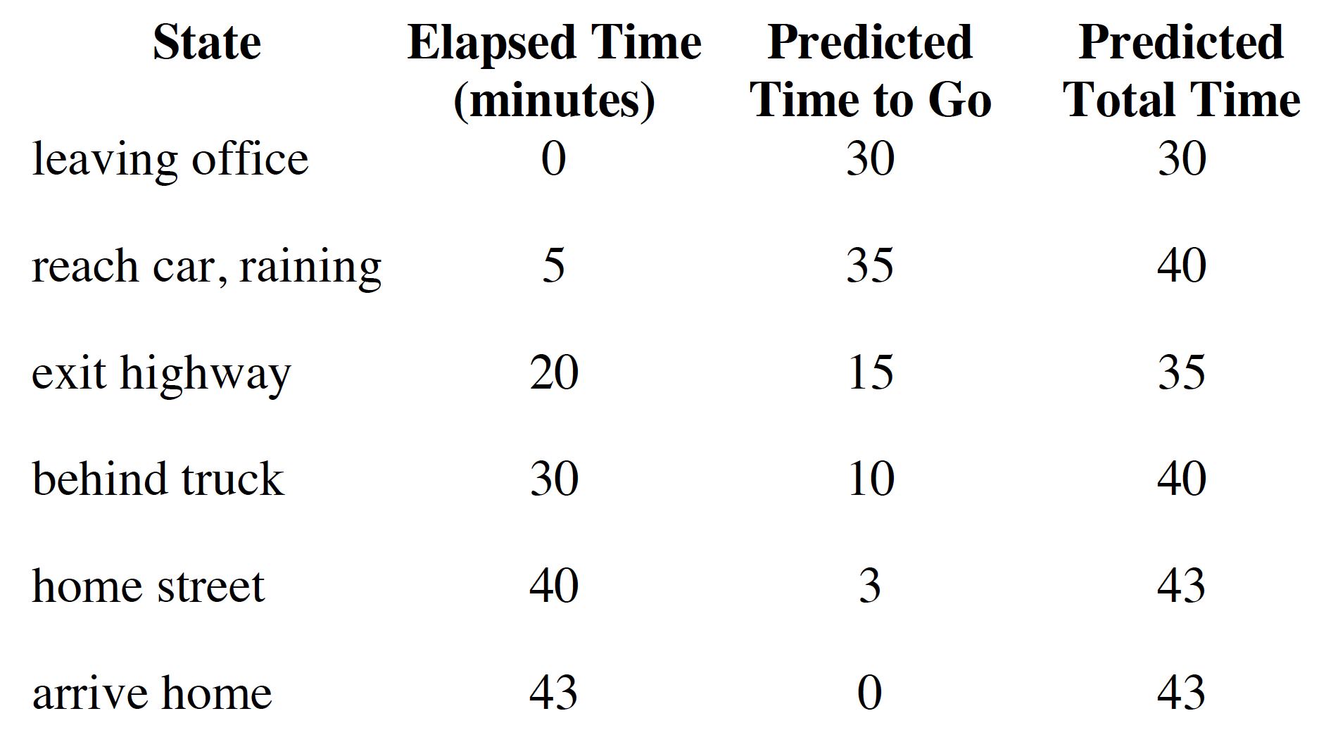
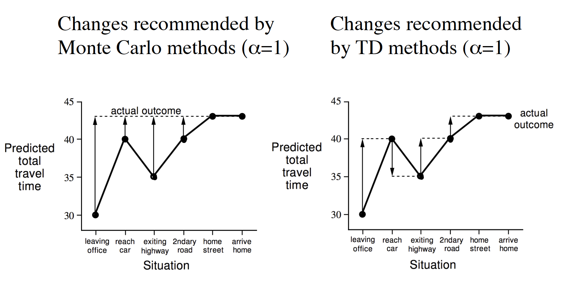
In the above picture, elapsed time shows the amount of time it took the agent to get to a particular state. As such, the driver exited the highway after 20 minutes and was home in 43 minutes. Predicted time to go is the time that the agent thinks it will take him to get to to the terminal state, “arrive home”, starting from the current state. For example, after the agent reached the car and realized that it was raining, he thought that it would take him 35 minutes to arrive home from that state. Finally, the predicted total time is the amount of time that the agent thinks it will take him to get home taking into account the time that has already passed, i.e. the total predicted time is the sum of elapsed time and the predicted time to go. Now think of the elapsed time as a realization from an episode, i.e. the actual elapsed time could be viewed as the realized reward. The predicted time to go then represents the value of each state. The diagram below shows how the two methods would update the state-value function.

1. TD can learn before knowing the final outcome. MC, on the other hand, must wait until the end of an episode when the return is known.

2. TD can learn without the final outcome. Thus, TD is applicable in continuing (non-terminating) environments. MC only works for terminating (episodic) environments.

3. Bias/Variance trade-off. The realized cumulative discounted reward from an episode, $G_t = R_{t+1} + \gamma R_{t+2} + \gamma^2 R_{t+3} + \cdots$, that is used in MC method, is an unbiased estimate of $v(S_t)$, the true value of state $S_t$. Even though $R_{t+1} + v(S_{t+1})$ is an unbiased estimate of $v(S_t)$, we do not know the true state values, i.e. we use the estimates $V(S_t)$ and $V(S_{t+1})$ in TD. The bias arises from the fact that $V(S_t)$ is not equal to $v(S_t)$. Thus our estimates are biased. On other hand, TD methods are lower variance. This is because $G_t$ depends on many random actions, transitions, rewards; while TD targets depend on one random action, transition and reward. In other words, if you were to run episodes starting from a given state $S_t$, your estimates from the MC method would show way more variation than the estimates from the TD method. In summary, MC method leads to unbiased estimates of the true state-value function at the cost of having higher variance:

   • Good convergence properties (even when using function approximation)
   • Not very sensitive to the initial values
   • Simple to understand and use

TD methods are lower variance but are biased: - Usually more efficient than MC method - TD converges to $v_{\pi}(s)$ (but not always with function approximation) - More sensitive to initial conditions

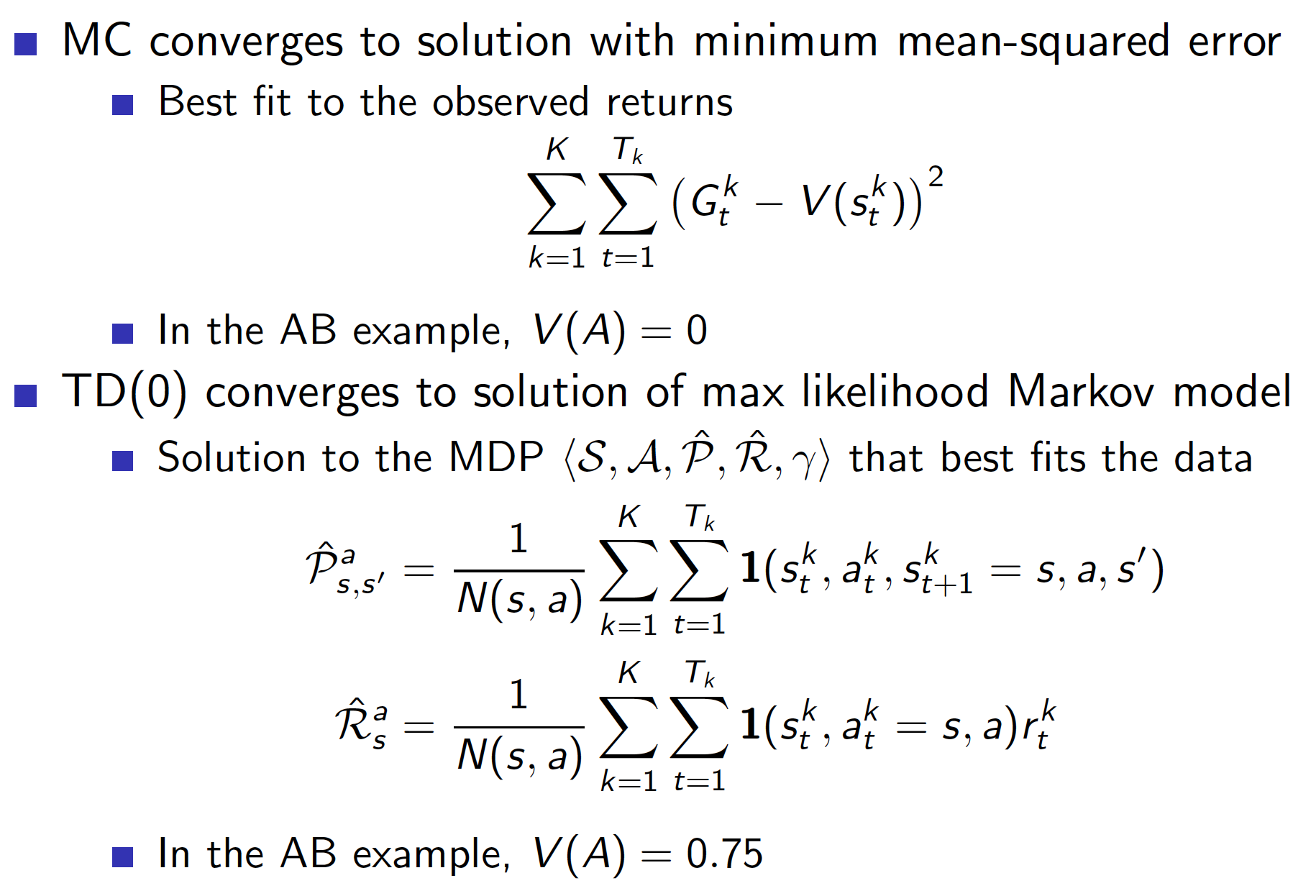
1. Both methods, MC and TD, converge to the true state-value function as the number of episodes of experience $\rightarrow \infty$. But what would happen if we had only a finite number of episodes and kept on training the two methods on them? For example, suppose we have the following realization from 8 episodes.

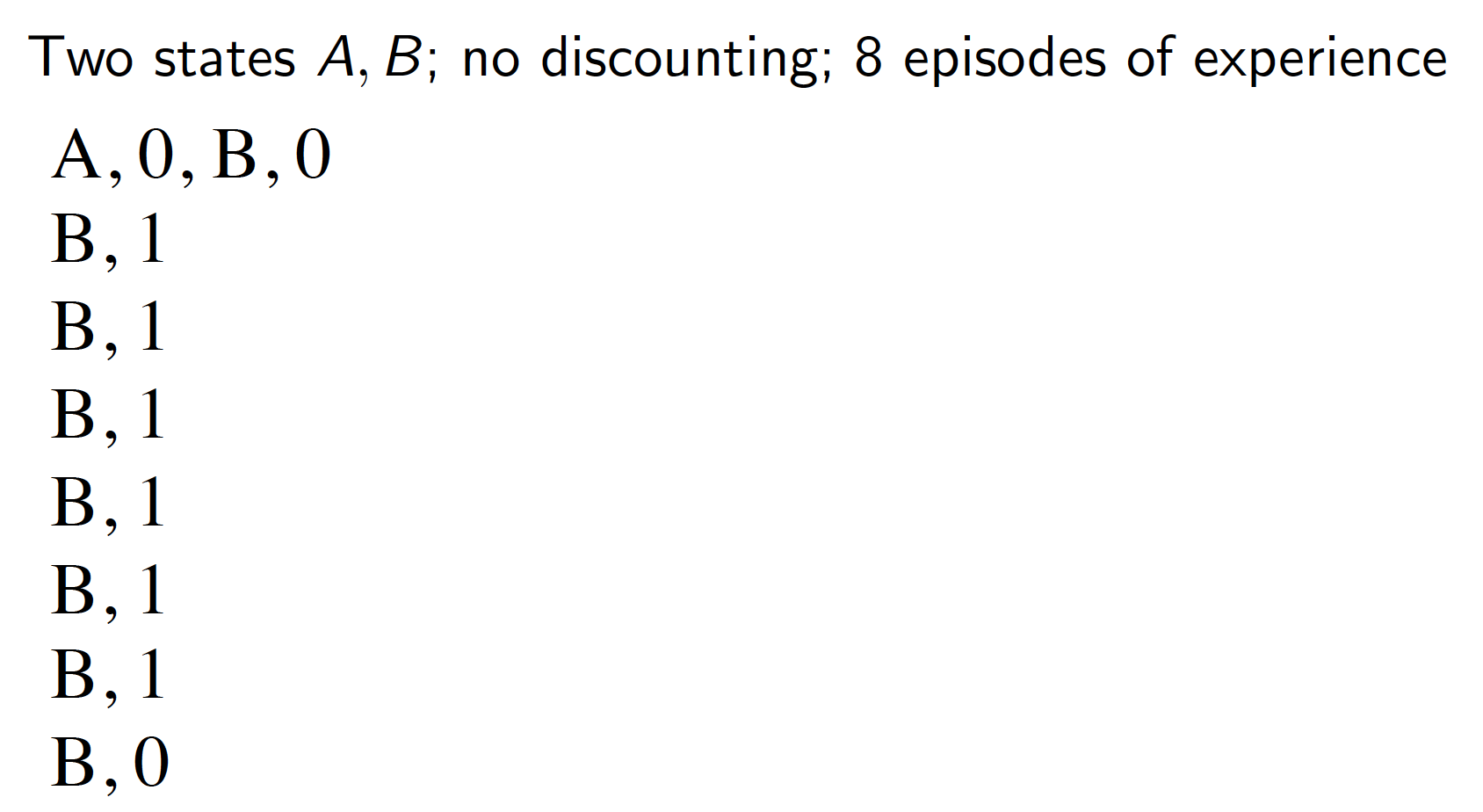
What is $V(A)$ learned by MC and TD methods respectively? MC converges to the solution with minimum MSE. So, $V(A) = 0$ in this case. TD converges to the solution of maximum likelihood Markov model. Hence, $V(A) = 1\times0.75 + 0 \times 0.25 = 0.75$.

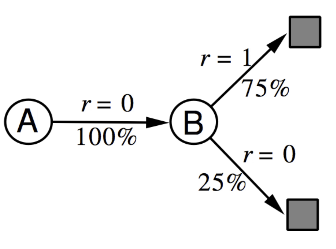
In other words, TD first finds the MDP model that best fits the data and the learned state-value function is the solution to that MPD. Expressed differently, TD converges to the solution of the MDP that best explains the data.

1. The TD method exploits the Markov property. This is because the TD method first tries to reconstruct the most likely MDP from which the observed data was generated and then solves that MDP. Consequently, TD methods work quite well in Markov environments. MC methods, on other hand, do not exploit the Markov property, which makes them better choices for non-Markov environments, e.g. partially observed states.

Backups / Updates

This section graphically summarizes the backups (updates) for the three methods of MDP prediction.

1. Monte-Carlo Method

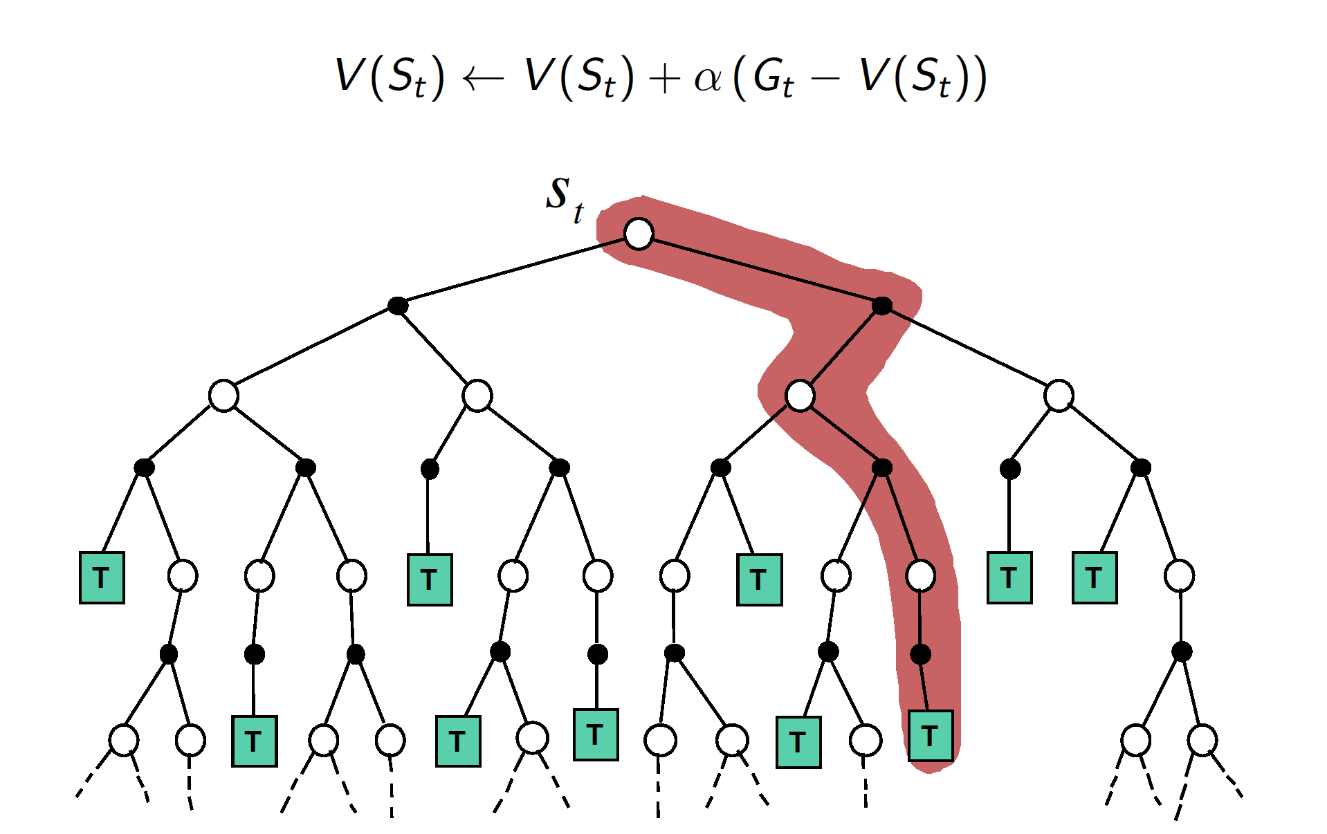
As the above graph implies, MC method works by sampling a terminating trajectory of realized returns and then updates the value of each state it visited along the way. Also, MC method does not bootstrap, i.e. it does not require any estimates but works with the actual returns instead.

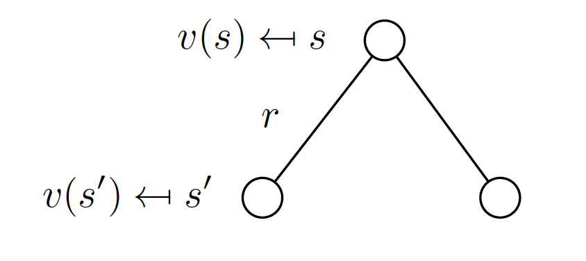
1. TD Method

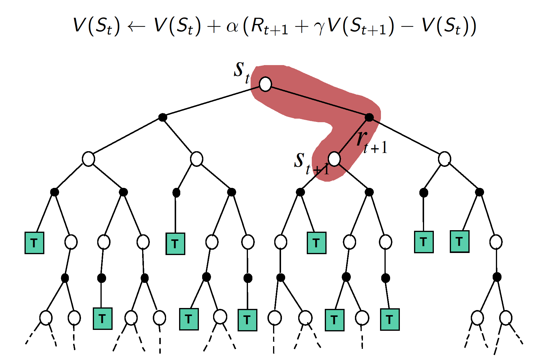
TD method, on the other hand, does not wait for a given episode to finish to start updating state values. In particular, TD method updates state values after each step. TD method uses bootstrapping, i.e. it works with estimates of the true state values to solve the problem.

1. Dynamic Programming

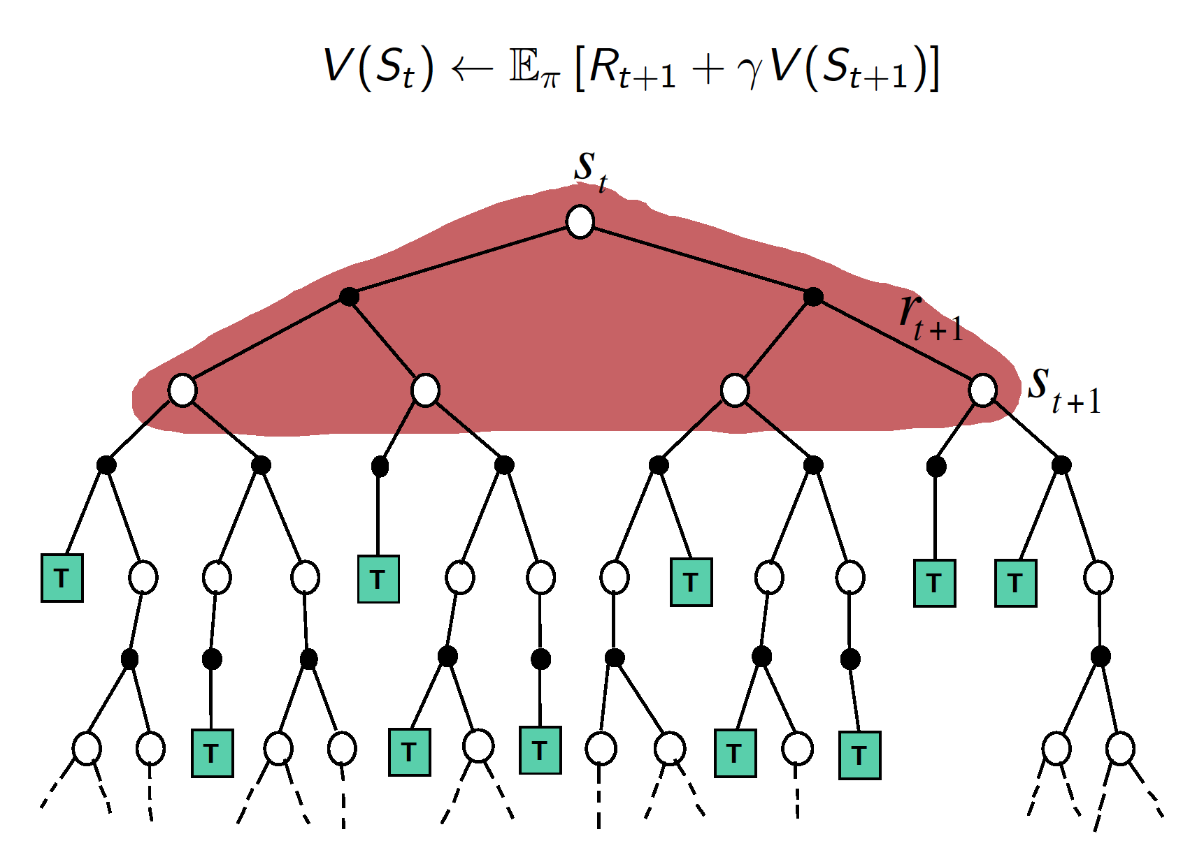
The dynamic programming approach updates state values taking into account all the possible state transitions and corresponding rewards. However, this is only possible if we are given the MPD, i.e. we know the reward function and state-transition probabilities. Similar to TD, DP methods use bootstrapping. Finally, unlike MC and TD methods, DP methods do not sample (this is not required as we have perfect knowledge of the dynamics of the MDP).

The picture below shows the unified view of the four methods.

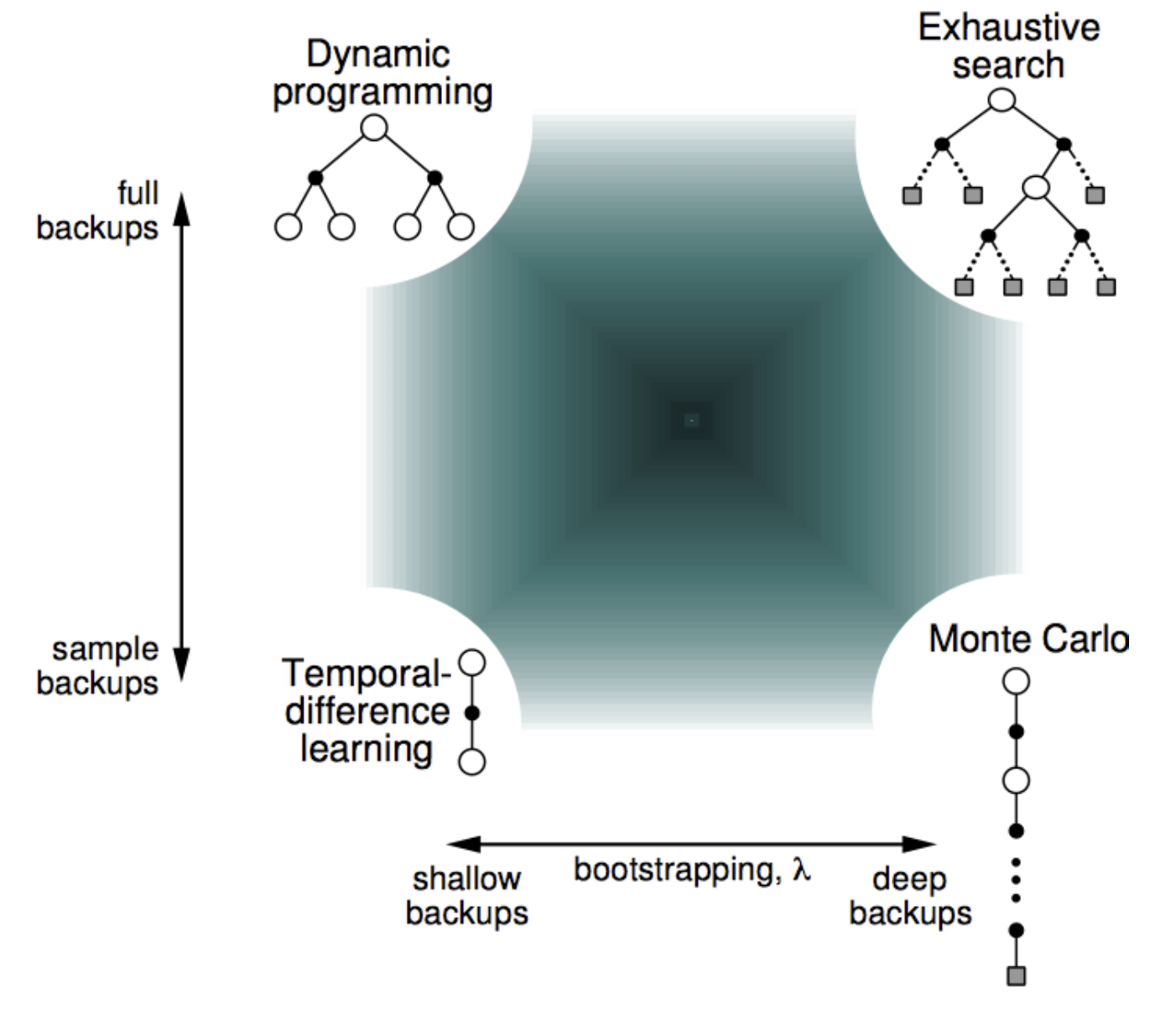
TD($\lambda$)

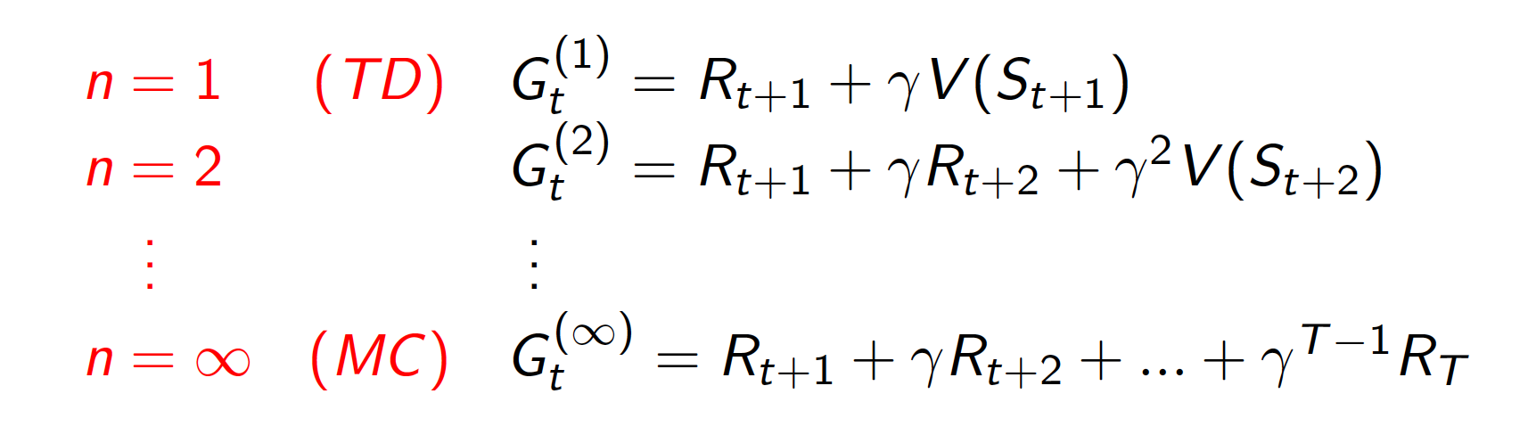
The graph above makes it clear that there is a whole different spectrum available for choosing between shallow and deep backups. Consequently, we can define the backup for an n-step TD method as

\[\begin{equation*} V(S_t) \leftarrow V(S_t) + a \left(G_t^{(n)} - V(S_t)\right), \end{equation*}\]

where

\[\begin{equation*} G_t^{(n)} = R_{t+1} + \gamma R_{t+2} + \gamma^2R_{t+3} + \cdots + \gamma^{n-1} R_{t+n} + \gamma^nV(S_{t+n}). \end{equation*}\]

Note that for sufficiently large $n$, we arrive at the MC method.

The question arises: What is the optimal choice of $n$ to be used in TD method? The short answer is: it really depends on the nature of the problem and the choice for other hyper-parameters. However, we can use information from all the different choices of $n$. In particular, observe that we can use the average of different $n$-step returns as our TD target. For example, we could use the average of two-step and four-step returns as follows:

\[\begin{equation*} \text{TD target} = 0.5 \times G_t^{(2)} + 0.5 \times G_t^{(4)}. \end{equation*}\]

As it turns out, we can use a geometric mean of all $n$-step returns in an approach called TD($\lambda$).

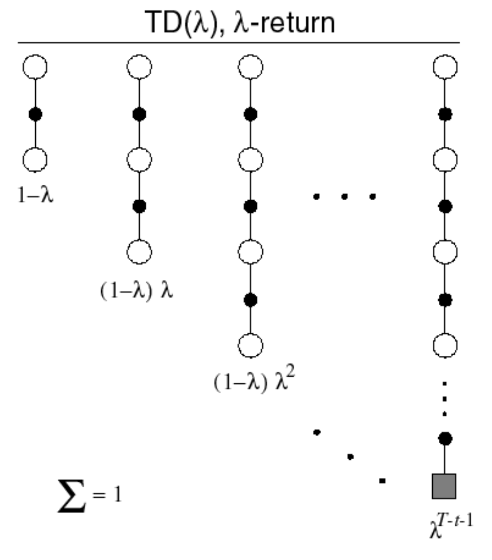
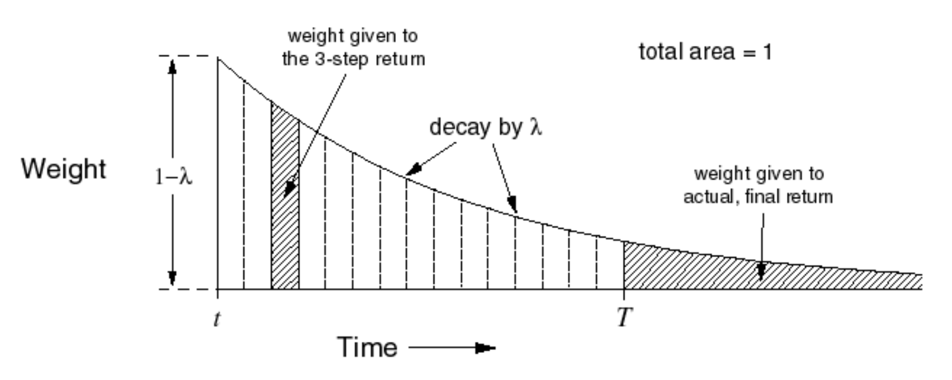
Note that the weight assigned to the return obtained from the final state can be larger (the total area should be equal to 1). The TD target is

\[\begin{equation*} G_t^{\lambda} = \left(1 - \lambda\right) \sum_{n=1}^{\infty} \lambda^{n-1}G_t^{(n)}. \end{equation*}\]

Our update equation becomes

\[\begin{equation*} V(S_t) \leftarrow V(S_t) + a \left(G_t^{\lambda} - V(S_t)\right). \end{equation*}\]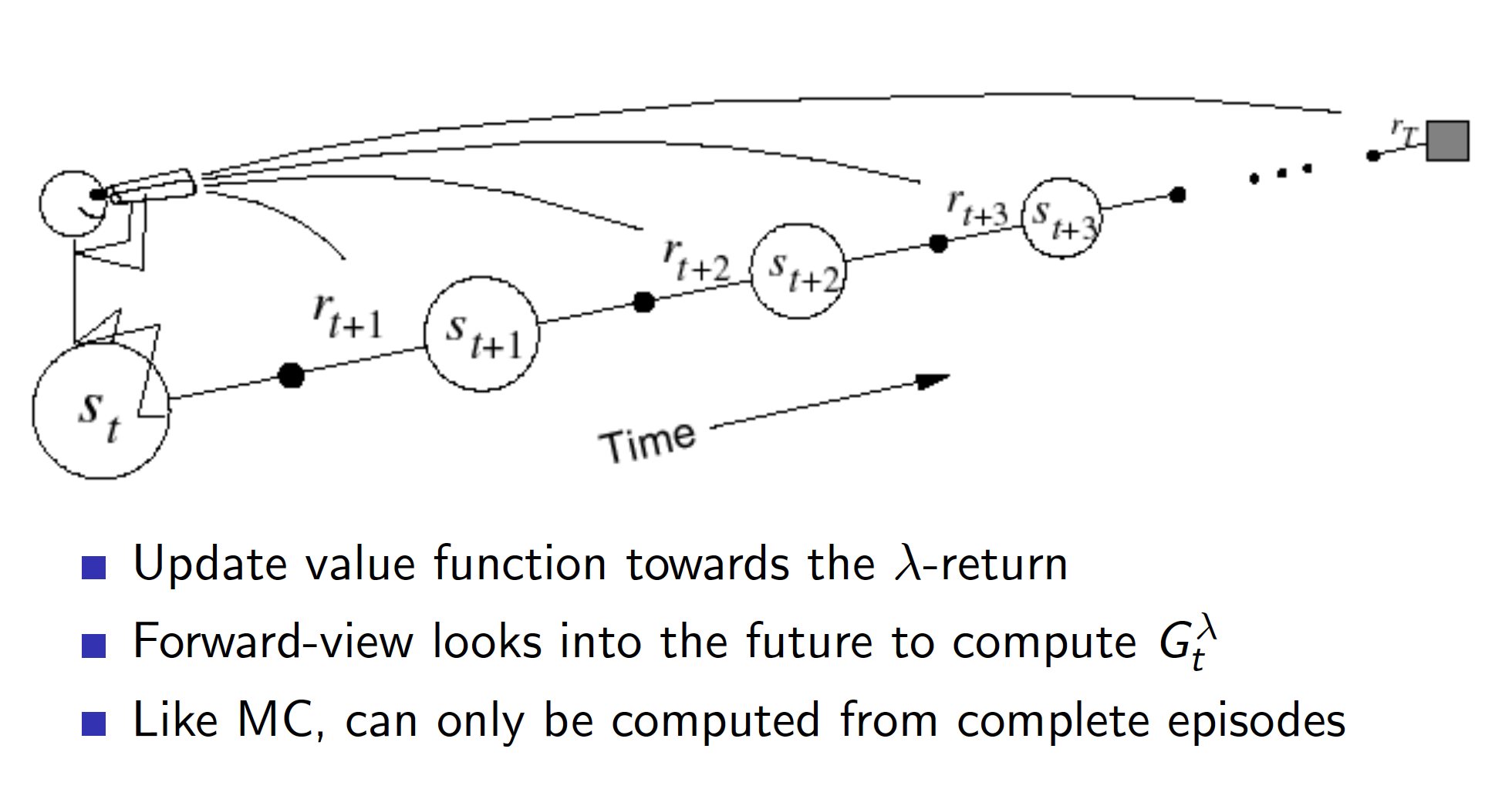

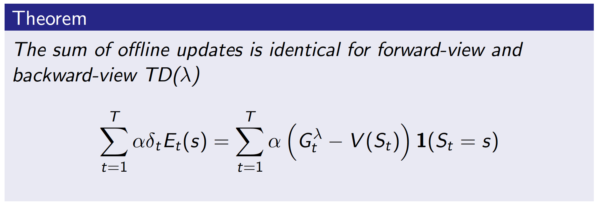
What we have discussed up to now is the forward or theoretical view of the TD($\lambda$) algorithm that allows us to mix backups to parametrically shift from a TD method to a MC method. The mechanistic, or backward, view of TD($\lambda $) is useful because it is simple conceptually and computationally. In particular, the forward view itself is not directly implementable because it is acausal, using at each step knowledge of what will happen many steps later. The backward view provides a causal, incremental mechanism for approximating the forward view and, in the off-line case, for achieving it exactly.

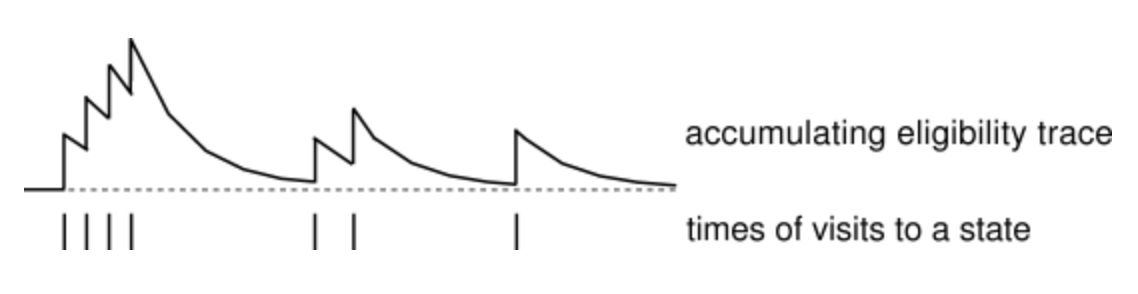
In the backward view of TD($\lambda $), there is an additional memory variable associated with each state, its eligibility trace. The eligibility trace for state $s$ at time $t$ is denoted $e_t(s)$. On each step, the eligibility traces for all states decay by $\gamma \lambda$, and the eligibility trace for the one state visited on the step is incremented by 1:

\[\begin{equation} e_t(s) = \begin{cases} \gamma \lambda e_{t-1}(s), \text{if $s \ne s_t$} \\ \gamma \lambda e_{t-1}(s) + 1, \text{if $s = s_t$}, \end{cases} \label{eq:eligibility_traces} \end{equation}\]

for all non-terminal states $s$. This kind of eligibility trace is called an accumulating trace because it accumulates each time the state is visited, then fades away gradually when the state is not visited, as illustrated below:

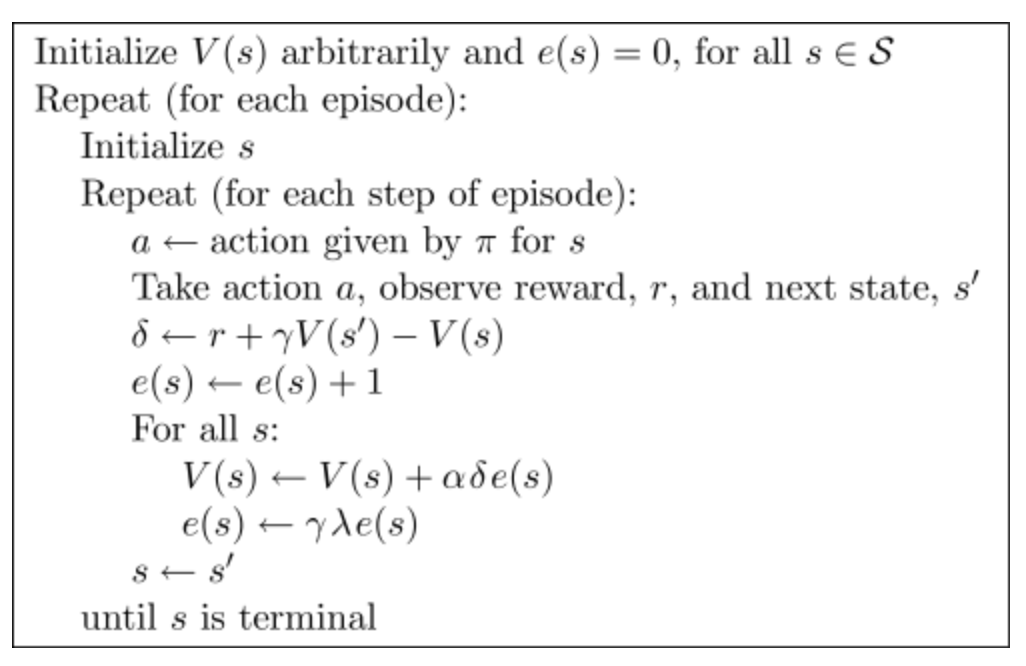
At any time, the traces record which states have recently been visited, where “recently” is defined in terms of $\gamma \lambda$. The traces are said to indicate the degree to which each state is eligible for undergoing learning changes should a reinforcing event occur. The reinforcing events we are concerned with are the moment-by-moment one-step TD errors. For example, the TD error for state-value prediction is

\[\begin{equation*} \delta_t = R_{t+1} + \gamma V(S_{t+1}) - V(S_t). \end{equation*}\]

In the backward view of TD($\lambda $), the global TD error signal triggers proportional updates to all recently visited states, as signaled by their nonzero traces:

\[\begin{equation*} \triangle V(S_t) = a\delta_t e_t(S_t). \end{equation*}\]

As always, these increments could be done on each step to form an on-line algorithm, or saved until the end of the episode to produce an off-line algorithm.

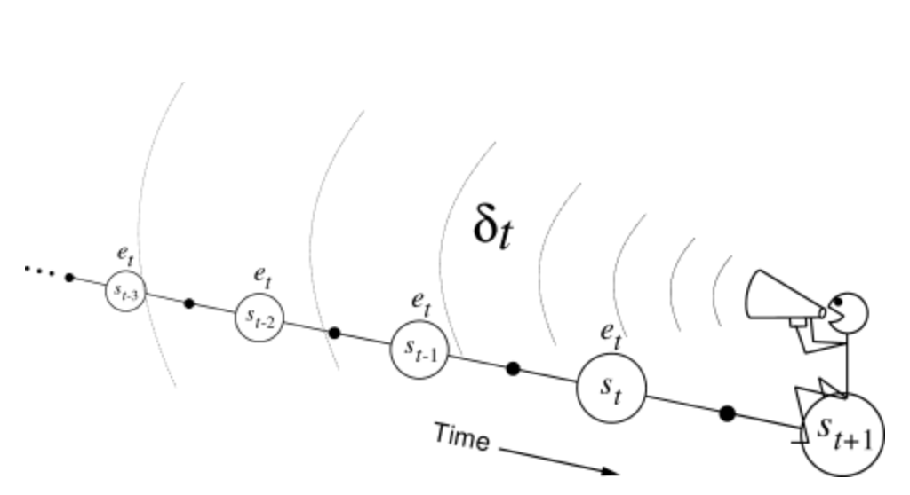
The backward view of TD($\lambda $) is oriented backward in time. At each moment we look at the current TD error and assign it backward to each prior state according to the state’s eligibility trace at that time. We might imagine ourselves riding along the stream of states, computing TD errors, and shouting them back to the previously visited states:

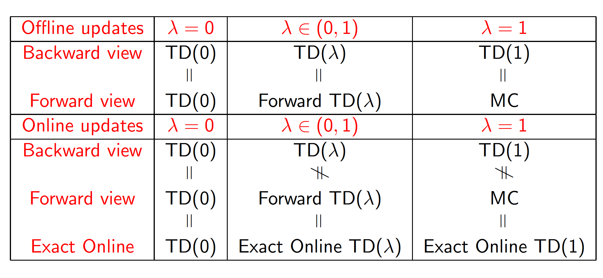
To better understand the backward view, consider what happens at various values of $\lambda $. If $\lambda=0$, then by Equation $\left(\ref{eq:eligibility_traces}\right)$ all traces are zero at $t$ except for the trace corresponding to $s_t$. Thus the TD($\lambda $) update reduces to the simple TD rule $\left(\ref{eq:TD(0)}\right)$, which we will call TD(0). TD(0) is the case in which only the one state preceding the current one is changed by the TD error.

For larger values of $\lambda$, but still $\lambda < 1$, more of the preceding states are changed, but each more temporally distant state is changed less because its eligibility trace is smaller, as suggested in the figure. We say that the earlier states are given less credit for the TD error.

If $\lambda=1$, then the credit given to earlier states falls only by $\gamma$ per step. This turns out to be just the right thing to do to achieve Monte Carlo behavior. Thus, if $\lambda=1$, the algorithm is known as TD(1). TD(1) is a way of implementing Monte Carlo algorithms that is more general than those presented earlier and that significantly increases their range of applicability. Whereas the earlier Monte Carlo methods were limited to episodic tasks, TD(1) can be applied to discounted continuing tasks as well. Moreover, TD(1) can be performed incrementally and on-line. One disadvantage of Monte Carlo methods is that they learn nothing from an episode until it is over. For example, if a Monte Carlo control method does something that produces a very poor reward but does not end the episode, then the agent’s tendency to do that will be undiminished during the episode. On-line TD(1), on the other hand, learns in an $n$-step TD way from the incomplete ongoing episode, where the steps are all the way up to the current step. If something unusually good or bad happens during an episode, control methods based on TD(1) can learn immediately and alter their behavior on that same episode.

Model-Free Control

In the previous lecture, we discussed model-free prediction, i.e. we asked our agent to evaluate (estimate state-value function) a given policy for an unknown MDP. In this lecture, we are going to address the problem of model-free control. In other words, we want our agent to find an optimal policy for an unknown MDP.

There are many real-world tasks that can be represented as an MDP. However, for most of them:

• MDP is unknown but we could sample observations and rewards, i.e. experience
• MDP is known but it is too complex to apply the techniques of dynamic programming to

In either case, model-free control techniques can be utilized.

On-policy learning means that we want to learn or evaluate some policy $\pi$ by following $\pi$. Off-policy learning, on the other hand, learns about policy $\pi$ by following a different policy or experience generated by some other agent. A good answer is available here.

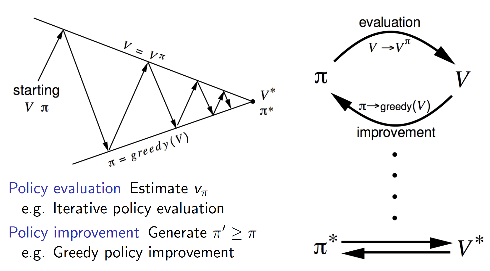
One of the main tools that we are going to use is the Generalized Policy Iteration that we saw in the lecture on Dynamic Programming. The idea of generalized policy iteration is to start with some policy, evaluate it and improve the policy by, for example, starting to act greedily with respect to that policy. This lecture is all about how we can evaluate and improve a given policy in a model-free environment.

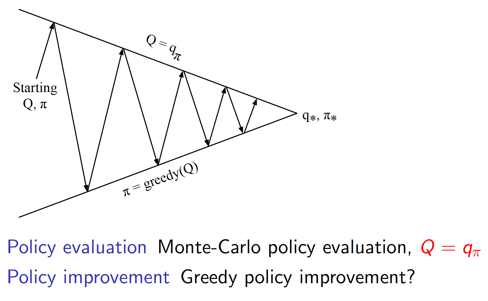
Monte-Carlo Control

For example, what would happen if we used Monte-Carlo policy evaluation (model-free prediction method discussed in lecture 4) and improved the policy by starting to act greedily with respect to the evaluated policy? Would that work? As it turns out, the answer is not. There are two problems with this approach:

• Since we have only evaluated the state-value function, there is no way for us to know how to act greedily with respect to the evaluated policy. We would need to know the state-transition function. In other words, greedy policy improvement over $V(s)$ requires model of MDP:

\[\begin{equation*} \pi'(s) = \underset{a\in A}{argmax}R_s^a + P_{ss'}^a(s'). \end{equation*}\]

Acting greedily with respect to the estimated/give state-value function requires knowledge of the MDP, i.e. it is not applicable in model-free environments. The alternative is to use the action-value function $Q(s,a)$. Greedy policy improvement over $Q(s,a)$ is model-free:

\[\begin{equation*} \pi'(s) = \underset{a \in A}{argmax}Q(s,a). \end{equation*}\]

The generalized policy iteration becomes evaluating the action-value function and then starting to act greedily with respect to that function.

Note that there is a problem remaining, the problem of acting greedily with respect to the evaluated action-value function. If he have not tried certain state and action pairs, we have no way of evaluating them. Thus, we may get stuck and never achieve the optimal behavior.

• There is a problem of exploration. We need to make sure that the agent explores the environment well and keeps on exploring throughout the learning process. The simplest approach (and very very effective) is $\epsilon$-greedy exploration. According to this technique, every action has a non-zero probability of being selected. That is,

\[\begin{equation*} \pi(a|s) = \begin{cases} 1-\epsilon + \frac{\epsilon}{m}, \text{if}\hspace{1.5mm} a = \underset{a \in A}{argmax}Q(s,a) \\ \frac{\epsilon}{m}, \text{otherwise}, \end{cases} \end{equation*}\]

where $m$ is the number of actions.

We have the following theorem:

Theorem: For any $\epsilon$-greedy policy $\pi$, the $\epsilon$-greedy policy $\pi’$ with respect to $q_{\pi}$ is an improvement, i.e. $v_{\pi’}(s) \ge v_{\pi}(s)$.

Proof: To show that the theorem is true, we need to show that acting greedily with respect to policy $\pi$ for a single step and then following $\pi$ is at least as good as following $\pi$ for a single step and for all the remaining steps. Hence,

\[\begin{align*} q_{\pi}(s, \pi'(s)) &= \sum_{a \in A}\pi'(a|s)q_{\pi}(s,a) \\ &= \frac{\epsilon}{m}\sum_{a \in A}q_{\pi}(s,a) + (1-\epsilon) \max_{a \in A} q_{\pi}(s, a) \\ &\ge \frac{\epsilon}{m}\sum_{a \in A}q_{\pi}(s,a) + (1-\epsilon) \sum_{a \in A}\frac{\pi(a|s) - \frac{\epsilon}{m}}{1 - \epsilon}q_{\pi}(s,a) \\ &= \sum_{a \in A}\pi(a|s)q_{\pi}(s, a) \\ &= v_{\pi}(s). \end{align*}\]

The above shows that the optimal value $q_{\pi}(s,a^*)$ of the optimal action $a^* = \max_{a \in A}q_{\pi}(s,a)$ taken with probability $1-\epsilon$ in state $s$ cannot be less than whatever the expected value is achievable by following the original policy $\pi$. For example, suppose that an agent is going to a food court everyday. He knows the values associated with choosing any given restaurant in the food court. Suppose that he follows some $\epsilon$-greedy policy $\pi$. Acting greedily with respect to this policy over a single step means that the agent will choose a random restaurant with probability $\epsilon$ and he will choose the restaurant with the highest value with probability $1-\epsilon$. The above expression basically states that this approach cannot be worse than choosing a random restaurant with probability $\epsilon$ and following $\pi$, regardless of what policy $\pi$ is, with probability $1-\epsilon$. Then, according to the policy improvement theorem (end of lecture 3), it follows that $v_{\pi’}(s)\ge v_{\pi}(s)$.

Combining Monte-Carlo policy evaluation with $\epsilon$-greedy policy improvement, we get the following Monte-Carlo control approach.

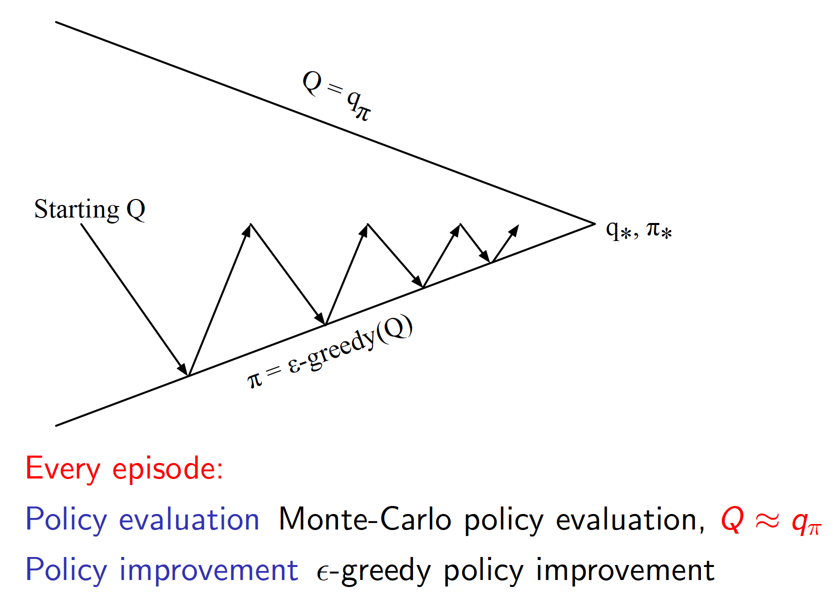
Note that it is not necessary to fully evaluate your policy before starting to act greedily with respect to it (that is why the arrows on the diagram above do not reach the top line). Put differently, we switch between policy evaluation and policy improvement steps more frequently. This makes the whole approach a lot more efficient.

Note that our final aim is to get $\pi^*$, i.e. an optimal policy for a given problem. So, throughout the learning process, we need to make sure than our agent keeps exploring the environment and taking different actions. At the same time, $\epsilon$, the rate of exploration, should be gradually reduced. The rationale is that an optimal policy is very unlikely to consist of taking random actions. Here we encounter an idea of Greedy in the Limit with Infinite Exploration (GLIE).

Definition (GLIE): A GLIE exploration schedule is the one that satisfies the following two conditions

1. All state-action pairs are explored infinitely many times

\[\begin{equation*} \lim_{k\rightarrow \infty}N_{k}(s,a) = \infty \end{equation*}\]

1. The policy converges to a greedy policy. In other words, the rate of exploration, $\epsilon$, converges to 0.

For example, GLIE Monte-Carlo control would work as follows:

• Sample $\text{k}^{th}$ episode following policy $\pi$ and observe ${S_1, A_1, R_1,\cdots, S_T}$
• For each state $S_t$ and action $A_t$ in the episode,

\[\begin{align*} N(S_t, A_t) &\leftarrow N(S_t, A_t) + 1 \\ Q(S_t, A_t) &\leftarrow Q(S_t, A_t) + \frac{1}{N(S_t, A_t)}\left(G_t - Q(S_t, A_t)\right) \end{align*}\]

• Improve policy and exploration rate as follows

\[\begin{align*} \epsilon &\leftarrow \frac{1}{k} \\ \pi &\leftarrow \epsilon-\text{greedy}(Q) \end{align*}\]

Theorem GLIE Monte-Carlo control converges to the optimal policy $\pi$, i.e. $Q(s,a) \rightarrow q^*(s,a)$.

TD Control

The natural way to improve our approach is to use TD methods instead of MC for policy evaluation. Remember that TD methods have certain advantages over MC methods:

• lower variance
• online learning
• can learn from incomplete sequences

Combined with $\epsilon$-greedy policy improvement, TD policy evaluation is one of the best RL algorithms ever developed. The general idea of this approach is known as SARSA.

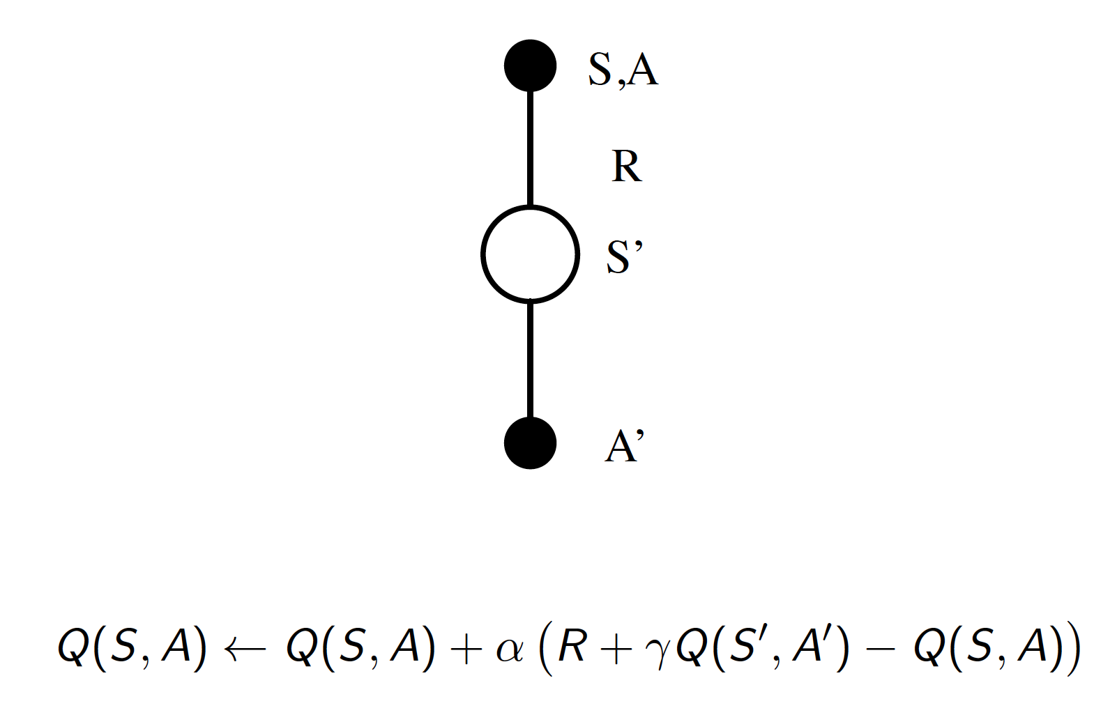
The approach to the control problem becomes

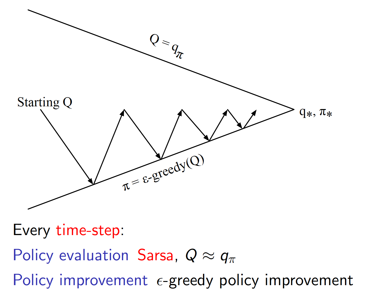
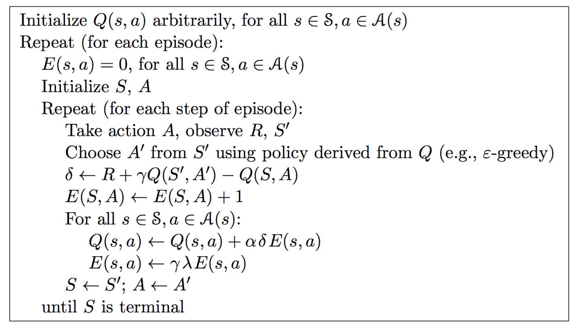
The complete SARSA algorithm for on-policy control would be

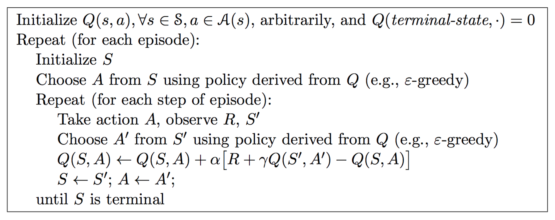
The following theorems states that SARSA converges to the optimal action-value value function provided that certain conditions are satisfied.

Theorem SARSA converges to the optimal action-value function, $Q(s,a) \rightarrow q^*(s,a)$ provided that the following conditions are satisfied:

• GLIE sequence of policies
• Robbins-Monro sequence of step-sizes $\alpha_t$, i.e.

\[\begin{align*} \sum_{t=1}^{\infty}\alpha_t &= \infty \\ \sum_{t=1}^{\infty}\alpha_t^2 & < \infty \end{align*}\]

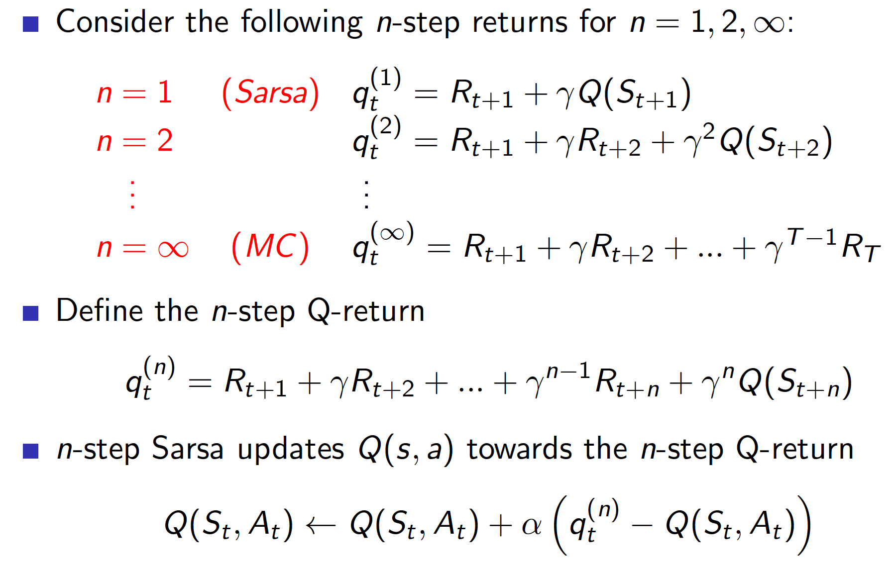
Similar to the previous lecture, we do not have to limit ourselves to only using a single TD step to evaluate our policy. Instead, we could use one of n-step returns. This would lead to an n-step SARSA approach.

To get the best of all the n-step returns, we can use SARSA($\lambda$) algorithm where we weight each of the n-step returns by $(1-\lambda)\lambda^{n-1}$. The diagram below gives the forward view (see lecture 4 about forward and backward views of TD($\lambda$) algorithm) of SARSA($\lambda$) algorithm.

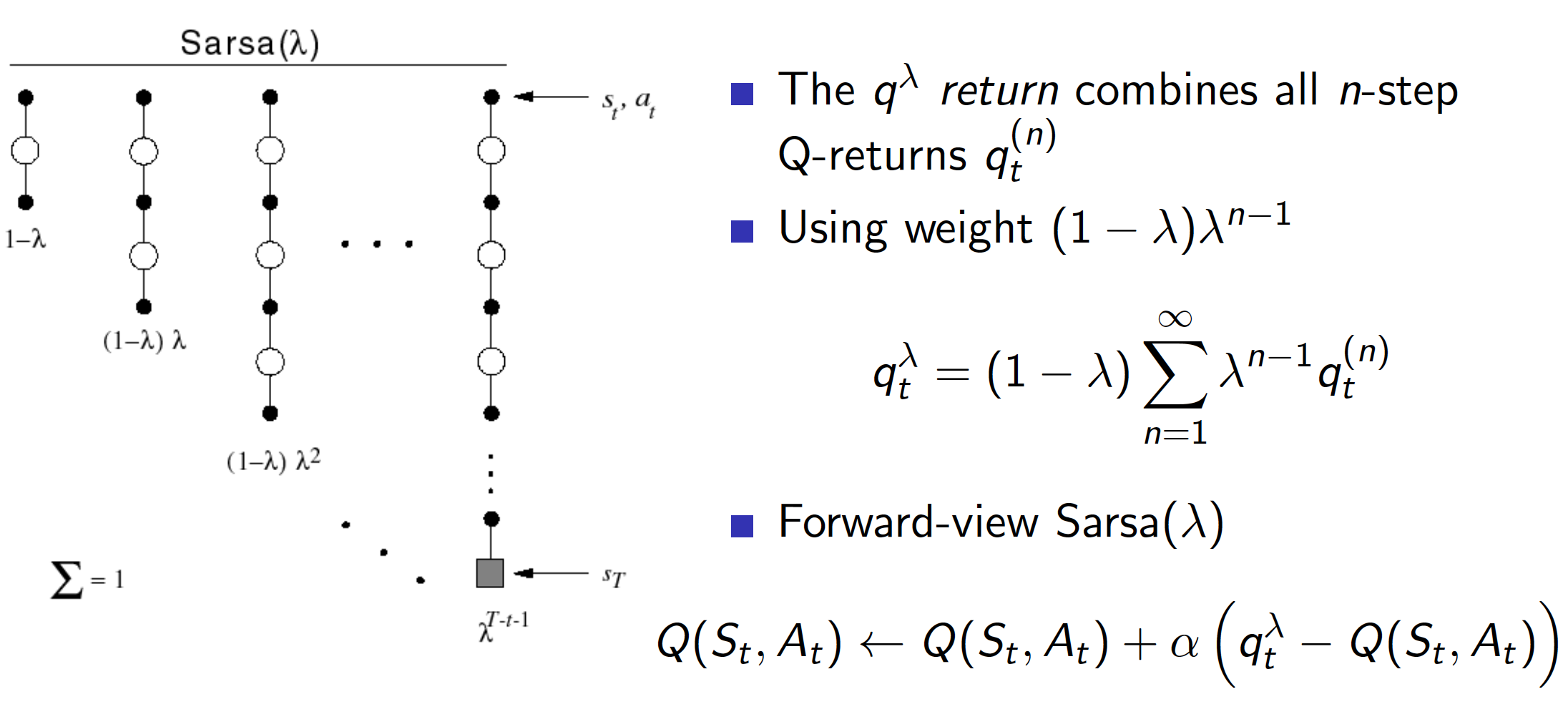
Similar to the forward view of TD($\lambda$) algorithm, the forward view of SARSA($\lambda$) algorithm just gives us an intuition. However, we cannot use the above in an online algorithm. To do that, we need the backward view.

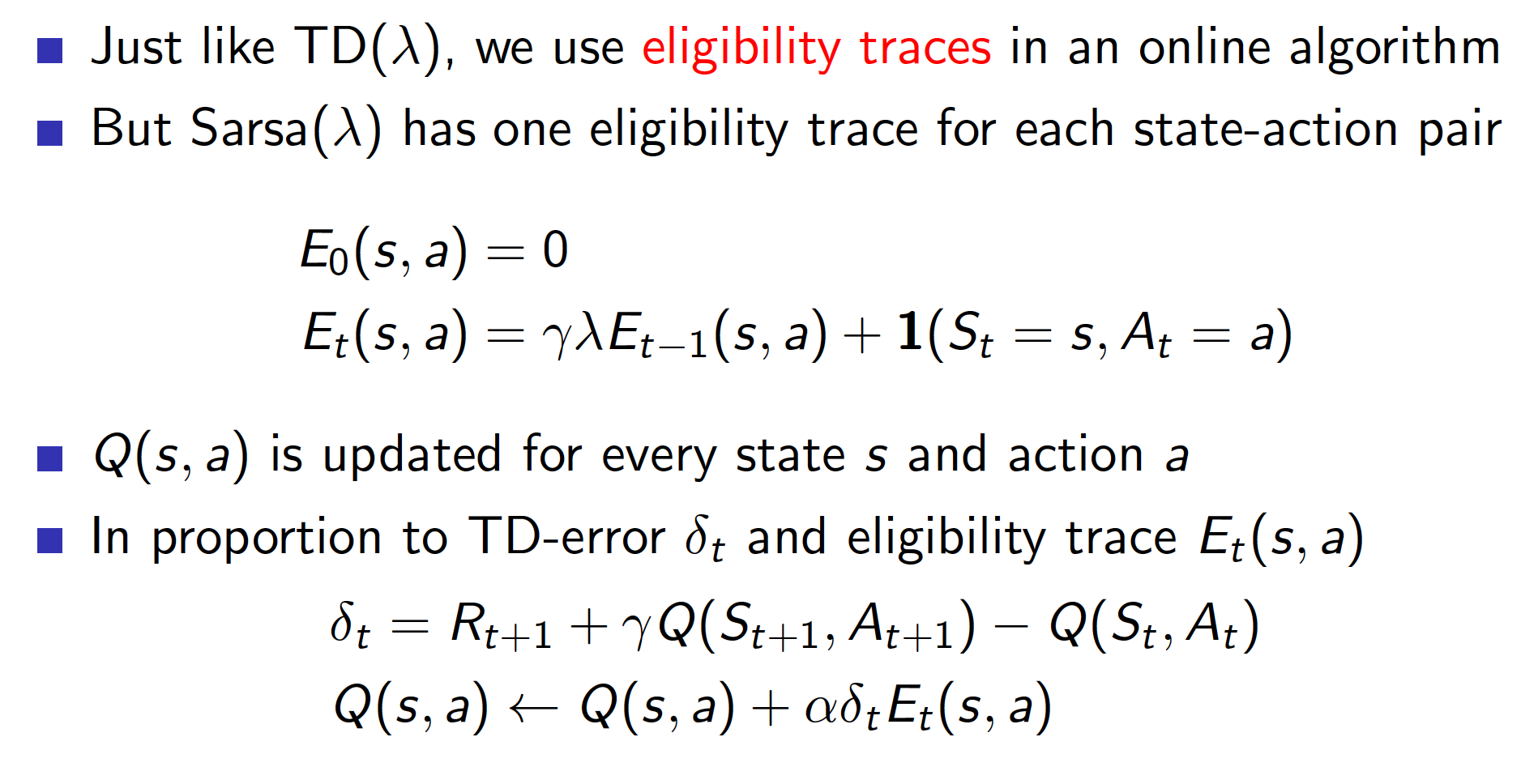
As a reminder, eligibility traces allow us to give proper credit to those states/actions that most likely led to whatever returns we are observing. In particular, state-action pairs that were visited recently and/or more often will be updated more than state-action pairs that were visited long time ago or very few times (if ever) when we observe our returns.

The actual algorithm is as follows.

The example below shows the difference between a single-step SARSA and SARSA($\lambda$) algorithms. In our example, assume that the agent receives 1 points in the final states and 0 elsewhere.

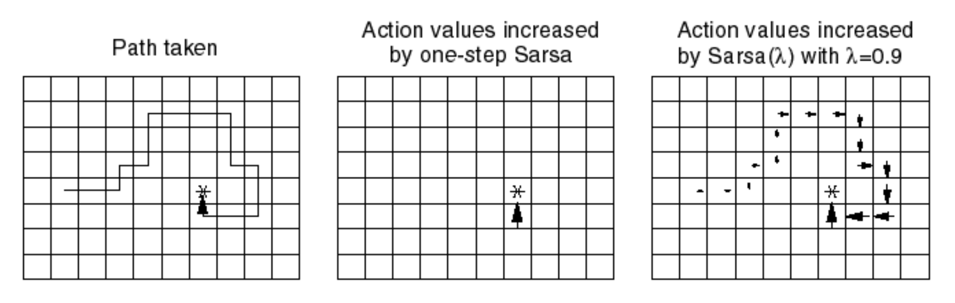
The leftmost image shows a realization of a single episode where the agent reached the target. In a single-step SARSA algorithm (middle picture), the whole credit would be given the state-action pair immediately preceding the winning square. In the SARSA(0.9) algorithm, all the state-action pairs taken/visited would be updated according to their corresponding eligibility traces. Note that the state-action pairs taken a long time ago would be updated less than more recent ones. $\lambda$ controls how far back and at what rate information is propagated back through state-action pairs taken/visited. When $\lambda=1$, we have Monte-Carlo control. We can see that SARSA($\lambda$) can potentially lead to faster learning as more state-action pairs get updated simultaneously.

Off-Policy Learning

In off-policy learning, we want to learn about some policy $\pi(a|s)$, i.e. either $v_{\pi}(s)$ or $q_{\pi}(a|s)$, by following some other policy $\mu(a|s)$. There are a number of reasons why we might want to use off-policy leaning:

• Our agent may learn by observing humans or other agents act in an environment
• Out agent can learn from prior policies $\pi_1, \pi_2, \cdots, \pi_{t-1}$, i.e. re-use experience from prior policies
• Learn about an optimal policy while following an exploratory policy
• Learn about multiple policies while following a single policy

One the central ideas of off-policy leaning is that of importance sampling. According to Wikipedia, “importance sampling is a general technique for estimating properties of a particular distribution, while only having samples generated from a different distribution than the distribution of interest”. For example,

\[\begin{align*} E_{X\sim P}\left[f(X)\right] &= \sum P(X)f(X) \\ &= \sum Q(X) \frac{P(X)}{Q(X)} f(X) \\ &= E_{X\sim Q}\left[\frac{P(X)}{Q(X)} f(X)\right]. \end{align*}\]

The equation above tells us that if we want to learn something about distribution $P$ but only have experience generated from distribution $Q$, we should adjust the experience by the ratio of the two distributions. Applying this idea to Monte-Carlo approach, we get

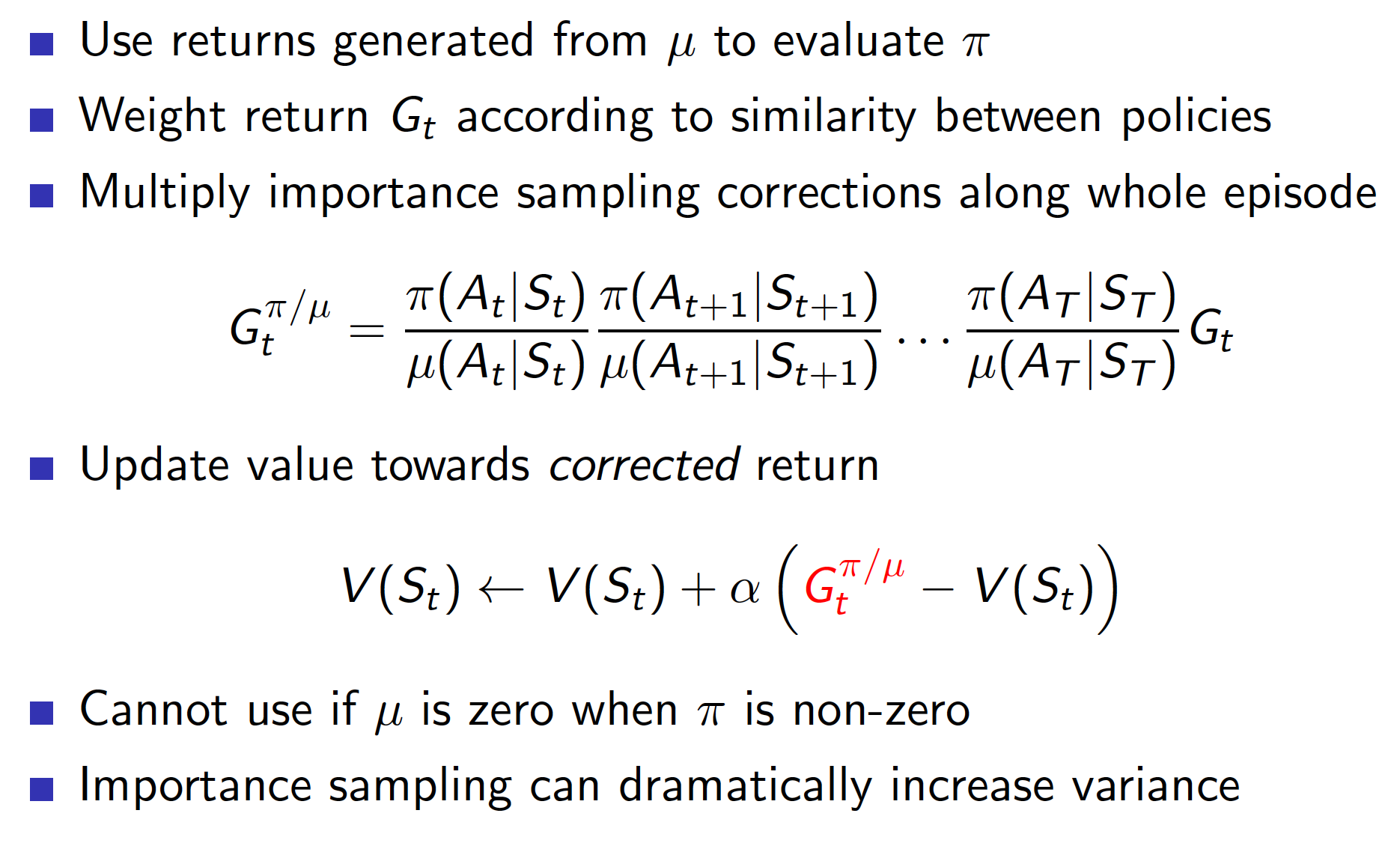
In practice, this is almost never used.

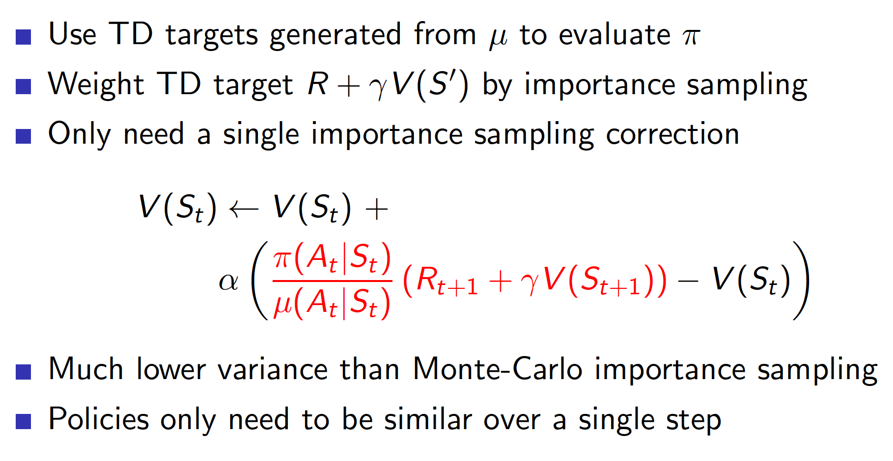
Off-policy TD, on the other hand, is much better.

However, off-policy leaning works best with Q-learning. No importance sampling is required at all. Very simply, we take actions according to policy $\mu(a|s)$. However, when we do bootstrapping, we generate the actions according to our target policy $\pi(a|s)$.

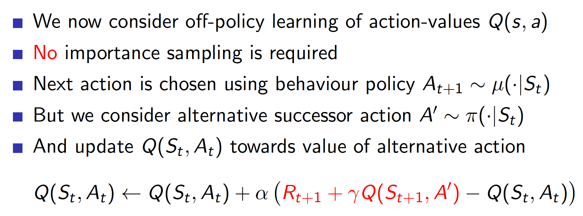
This is actually the idea behind the most common Q-learning algorithm (the one that you have always been using up to now without knowing it).

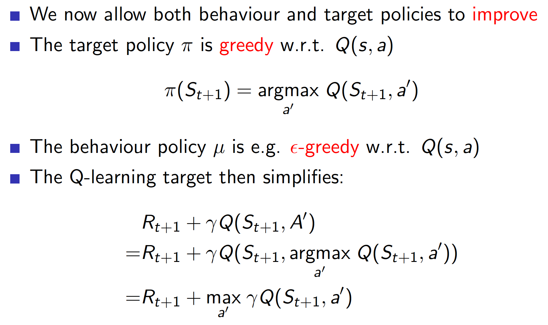
Basically, the above tells us that we can take actions according to an $\epsilon$-greedy policy (to explore the environment) but update the q-values of our target policy that has no random component any more. The following theorem does confirm that under this approach we will eventually reach an optimal policy.

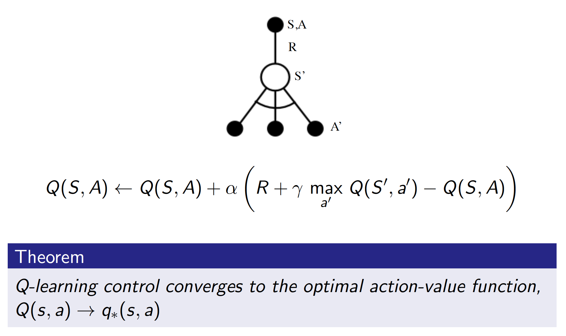
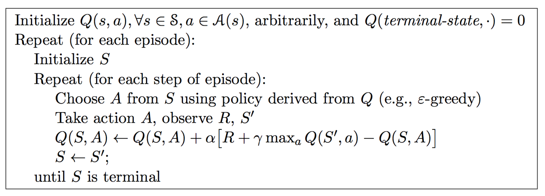
The algorithm is

Relationship between Dynamic Programming and Temporal Difference Learning

To summarize, below we show what relationships exist between DP approaches and TD learning.

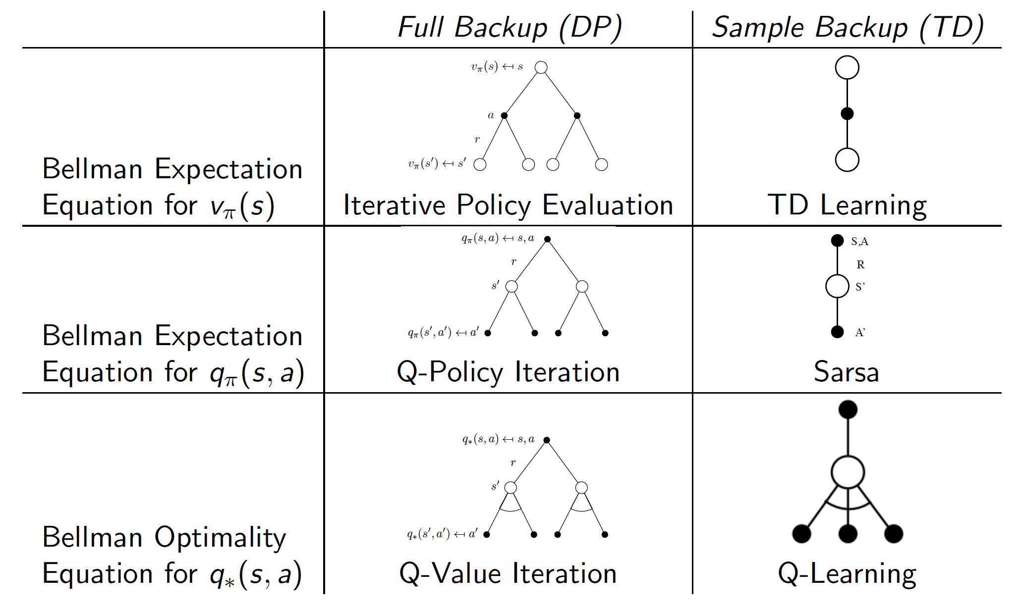
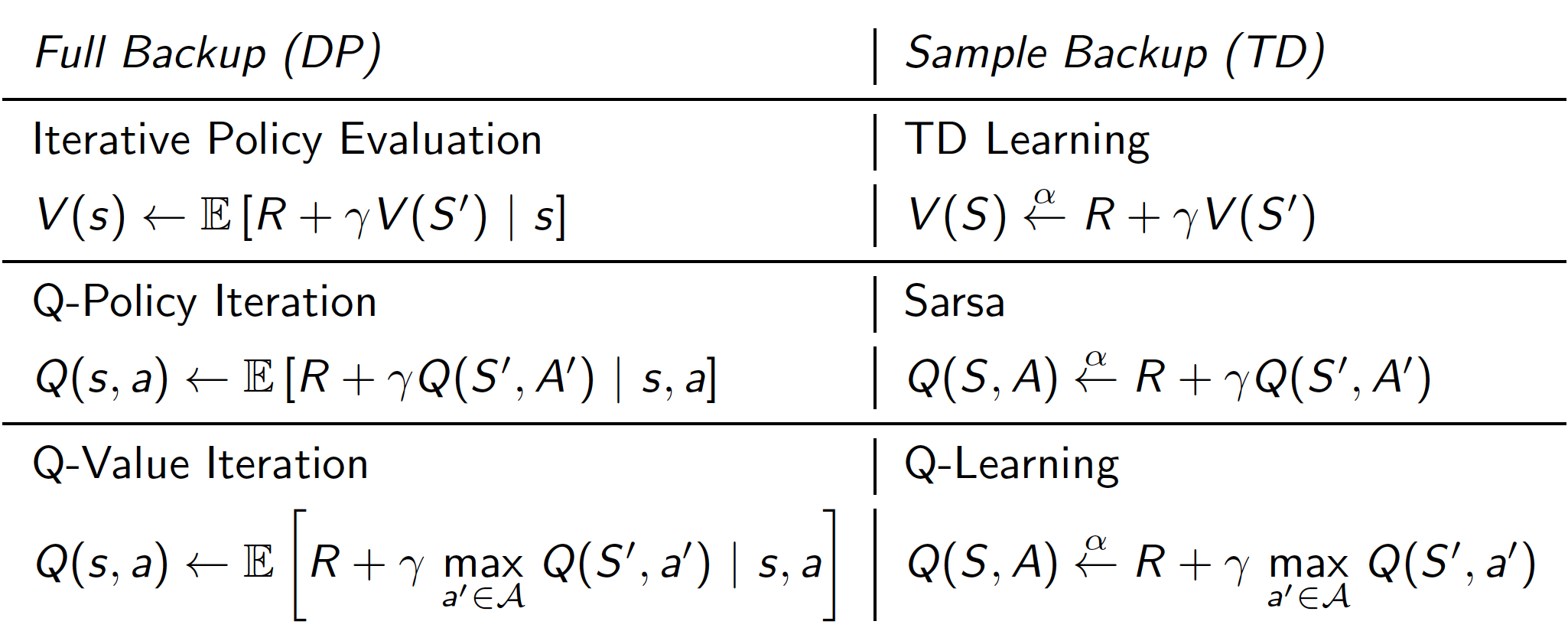
Note that

• DP techniques require that we know the dynamics of the underlying MDP (that is why have an expectation operator in the update equations). When these are unavailable, i.e. for most realistic problems, we have to use sampling techniques.
• The difference between SARSA and Q-learning is that the latter is an off-policy learning algorithm.

Value Function Approximation

Everything that we did up to now could have been done with table methods, i.e. all the value functions, both state and state-action, and eligibility traces could have been represented as vectors or matrices. However, table methods cannot deal with large-scale problems with many states and actions (most of real-life RL problems). The potential problems are:

• Table methods require too much memory to store values associated with each state or state-action pair.
• Learning becomes very inefficient as we update each individual entry in a value or Q-value table separately. However, intuitively, we should expect states that are “close” to each other to have similar values associated with them.

The solution to the scaling problem to use function approximations. In particular,

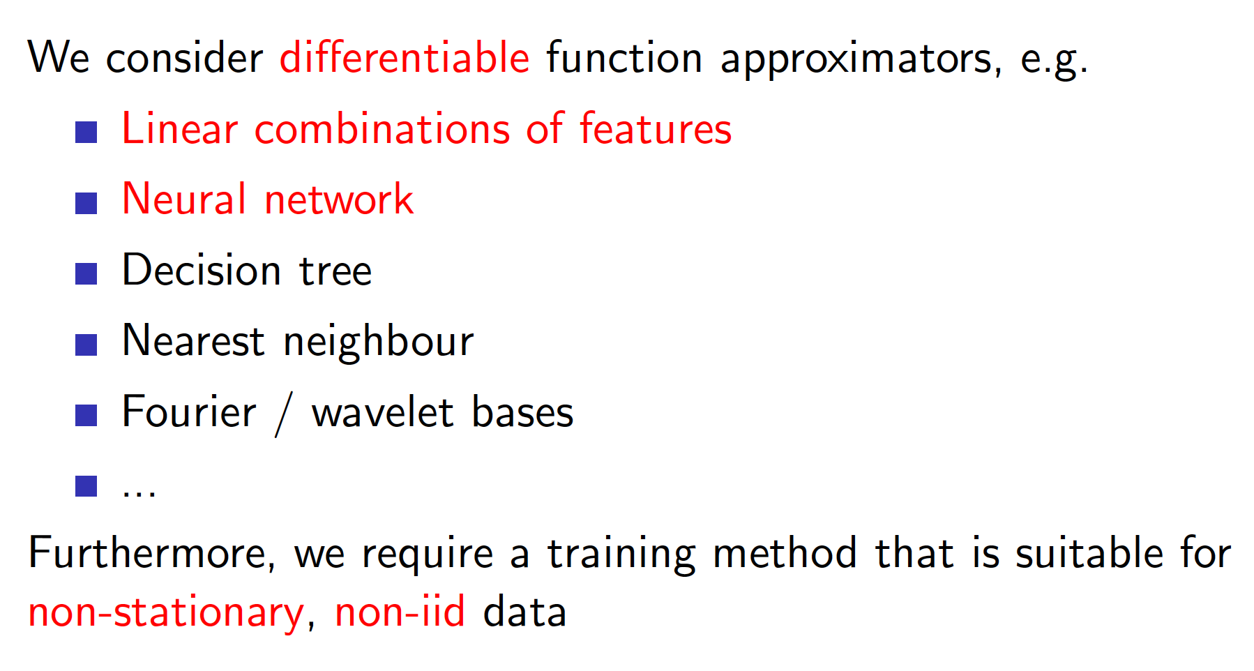
\[\begin{align*} \hat{v}(s, w) &\approx v(s) \\ \hat{q}(s, a, w) &\approx q(s,a). \end{align*}\]

The idea is then to construct a function that will approximate the true value or state-action value function with fewer parameters ($w$) than the number of states or state-action pairs. The use of function approximation will also allow us to generalize, i.e. we can approximately learn the values of states / state-action pairs even if we never visited them during training. We can use the techniques of MC and TD learning developed in preceding lectures to update the parameters of our function approximators. Note that there are many different function approximators that can be used.

Also, we may want our function approximators to approximate different value functions.

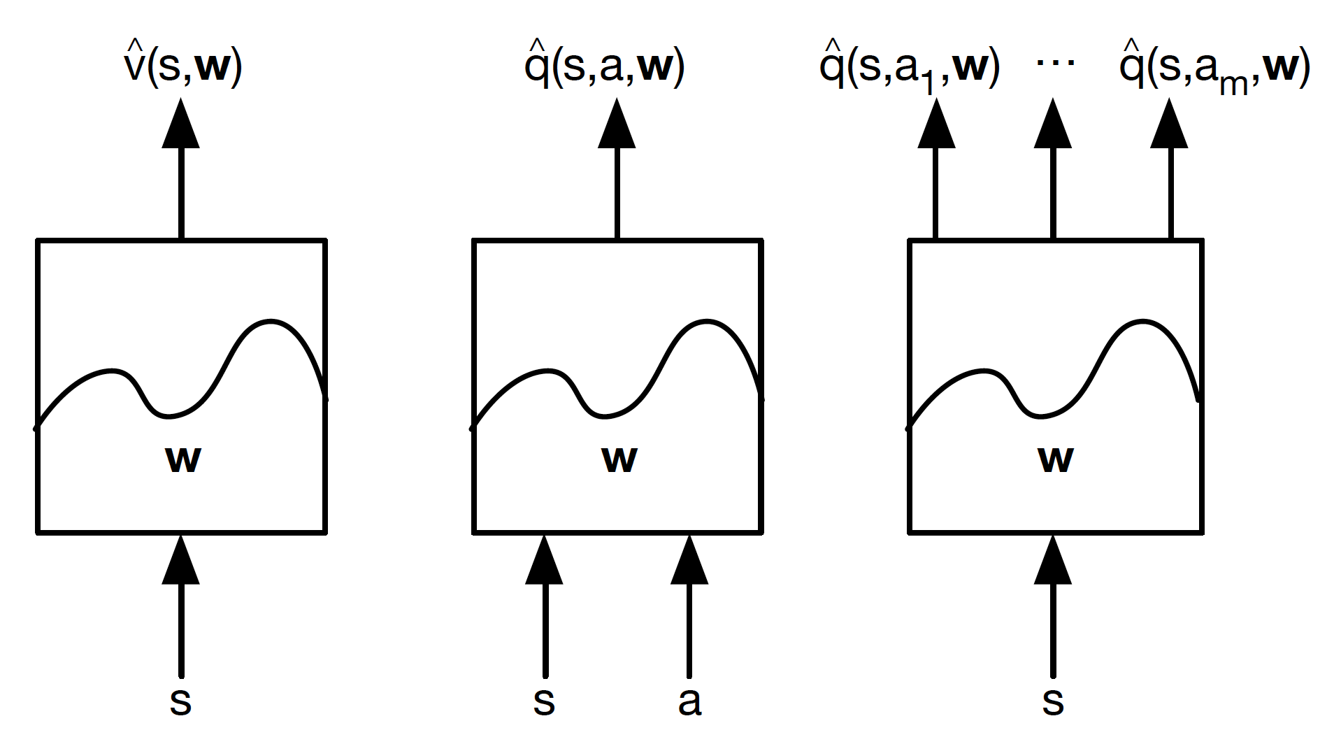
The leftmost type outputs the value of a given state. The middle one provides a Q-value associated with a state-action pair. Finally, the rightmost type is given a state and outputs an action value associated with each possible action in this state.

Incremental Methods

Since we are using differentiable function approximators, like Neural Networks, we should be familiar with Stochastic Gradient Descent (SGD) algorithm.

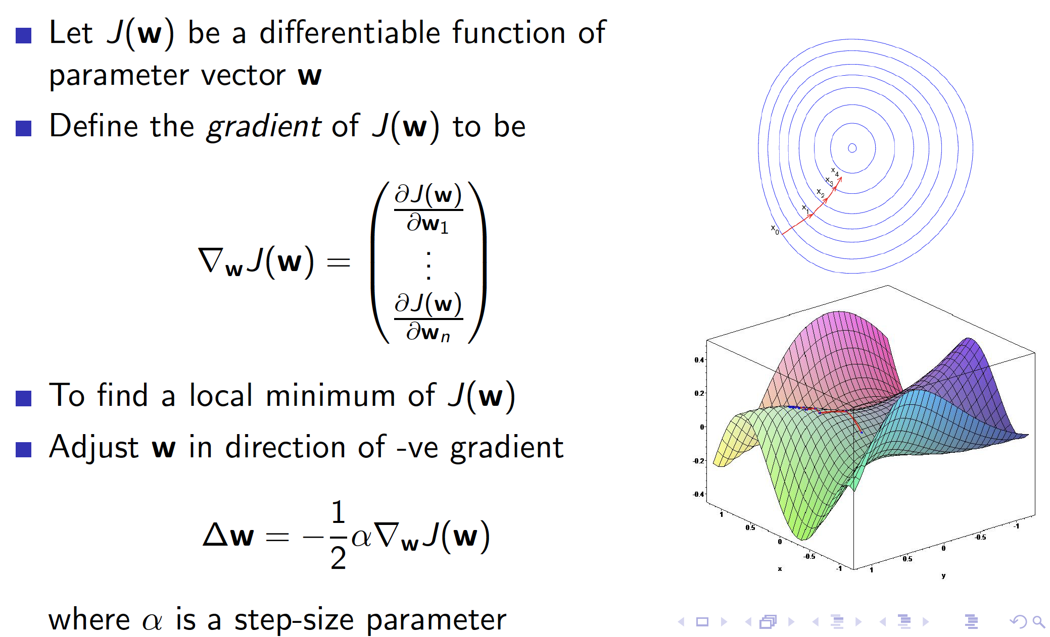
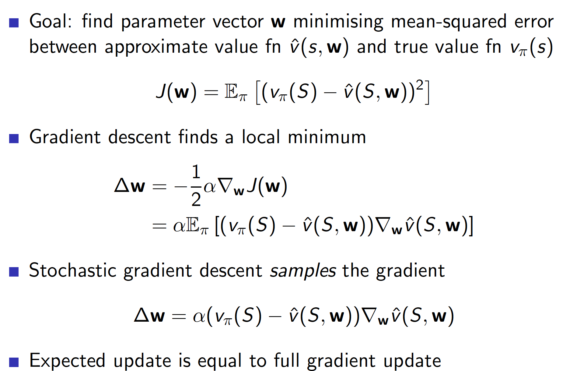
The goal of SGD is to find those weights that minimize the mean squared error (MSE) between the predictions and the true value.

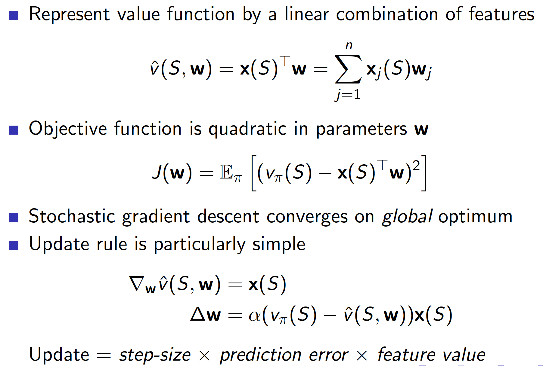
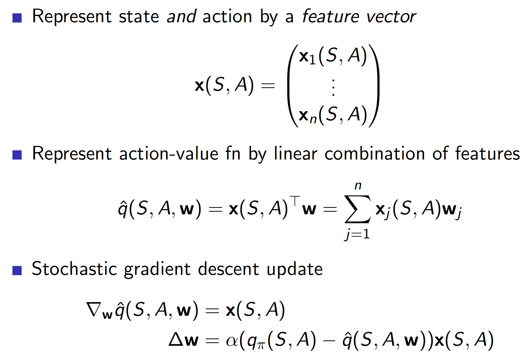
Feature vectors/matrices are constructed to provide a summary/representation of a given state.

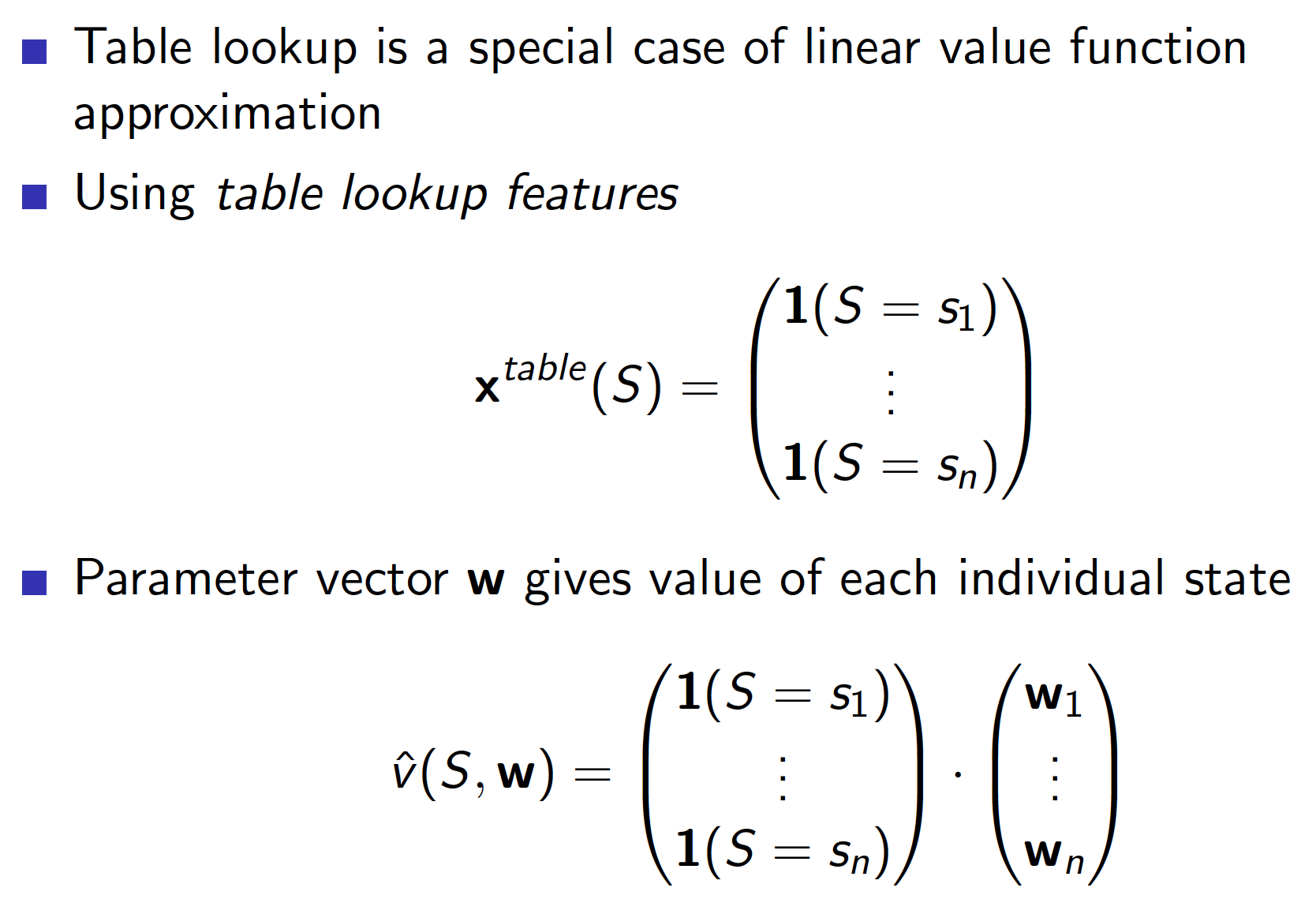
It is interesting to note that the table methods we considered up to this lecture are a special case of linear function approximation. In particular, if we consider a feature vector that consists of indicator functions for each of the possible states in an environment, we would get a table lookup method.

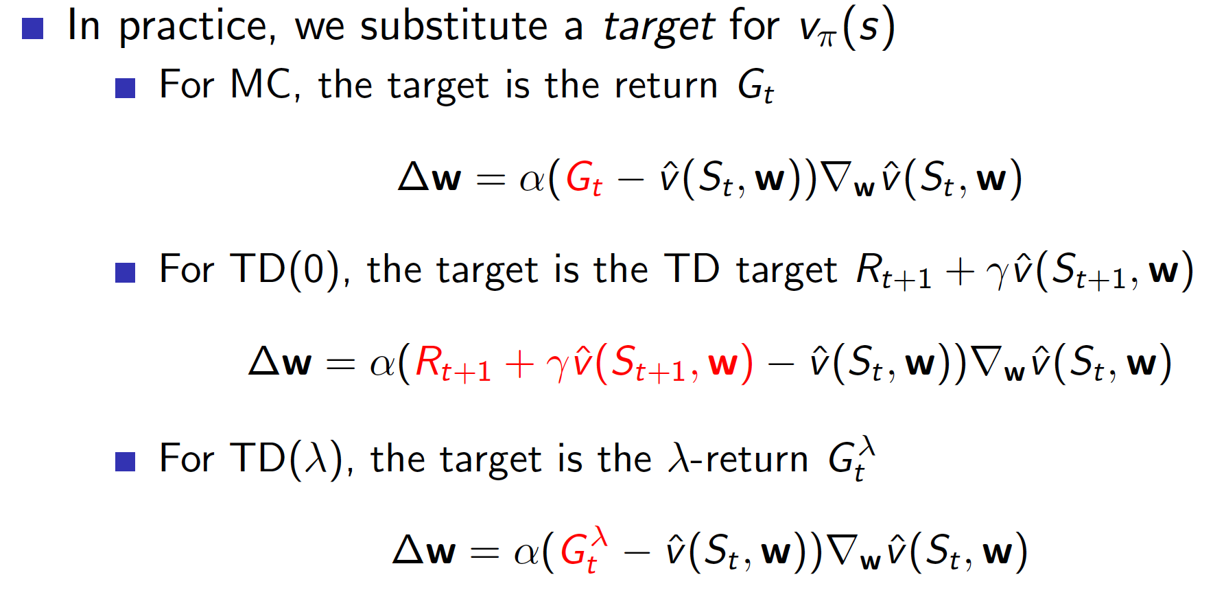
When we introduced SGD algorithm, we assumed that the true value functions are given to us (similar to a supervised learning setting). However, in practice, this is not the case in RL. Instead of using the true value functions, which are anyways not available to us, we should be using MC, TD and TD($\lambda$) targets that we discussed in previous lectures.

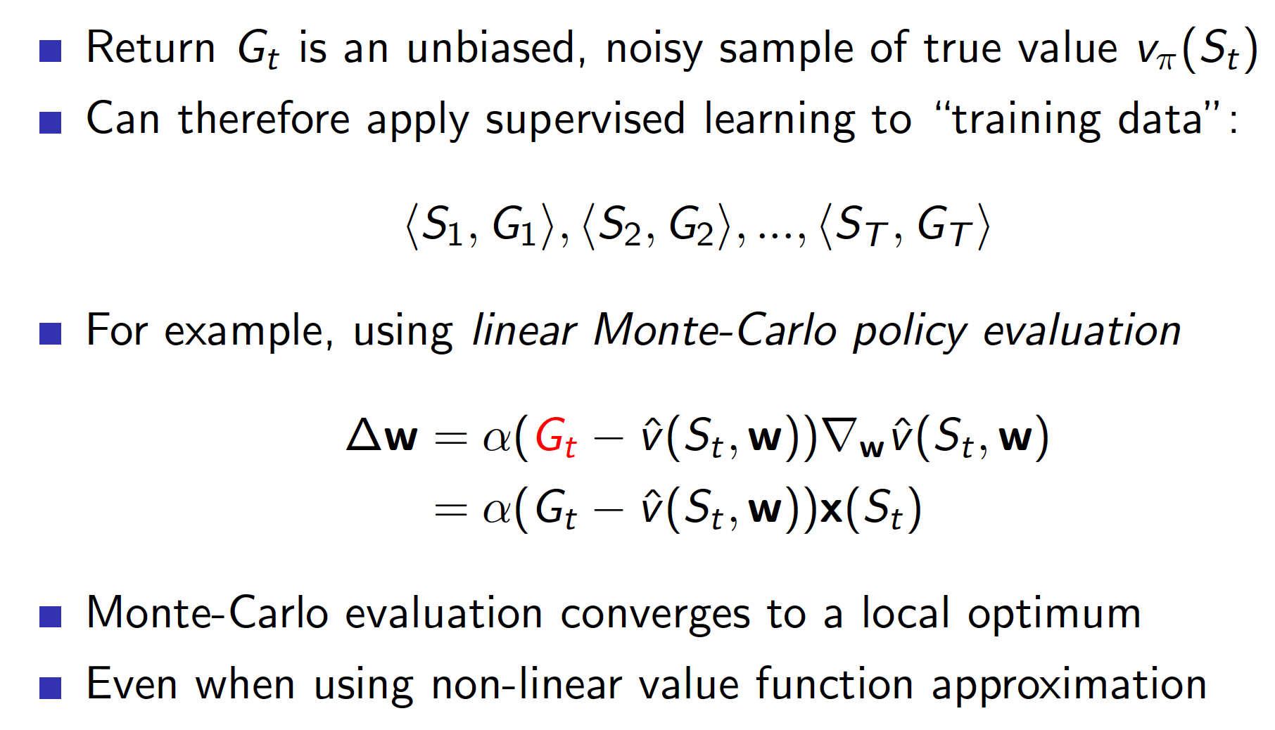
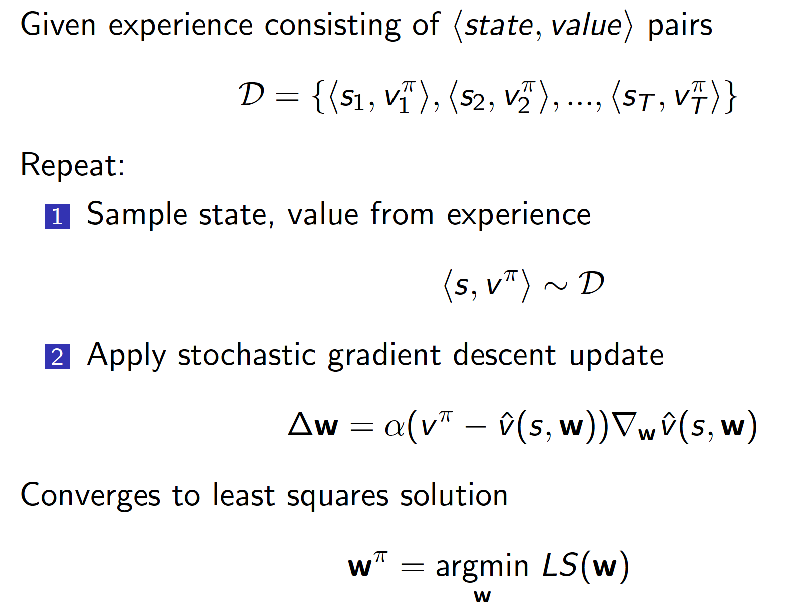
Monte-Carlo with Function Value Approximation

To implement Monte-Carlo method using function value approximation, we would run an episode of experience and collect realized returns. We would then proceed by fitting our function approximator to the obtained dataset (in a supervised learning fashion).

TD Learning with Function Value Approximation

TD learning with value function approximation is implemented in a similar way as MC with function value approximation. However, we do not have to play a full episode before starting to learn/estimate our value function (we could play a full episode(s) to collect a dataset for “supervised”-type learning but this will be covered in the subsequent part of the lecture). Also, our TD target is a biased estimated of the true value. This is because we are using our own value function approximator to derive the target.

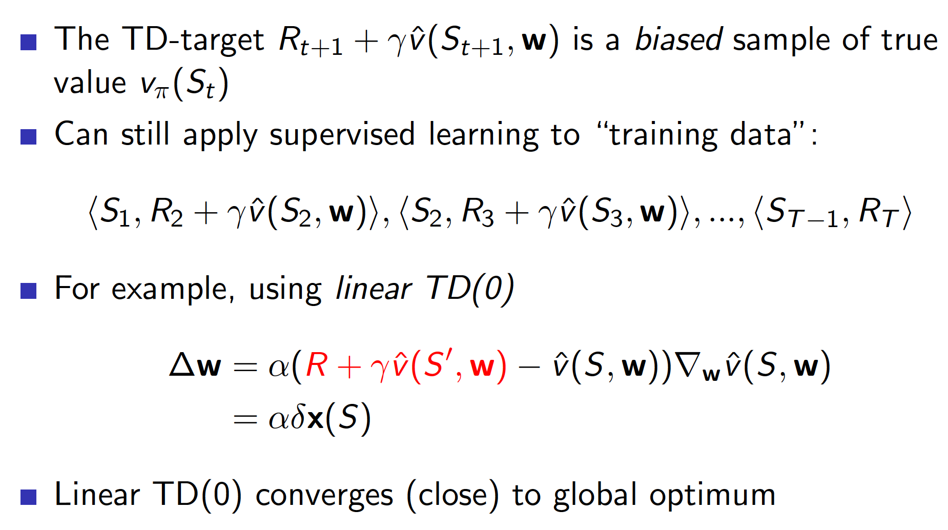
Note that even though our TD target is biased, TD(0) still converges closely to global optimum in the linear case, i.e. when our function approximator is linear.

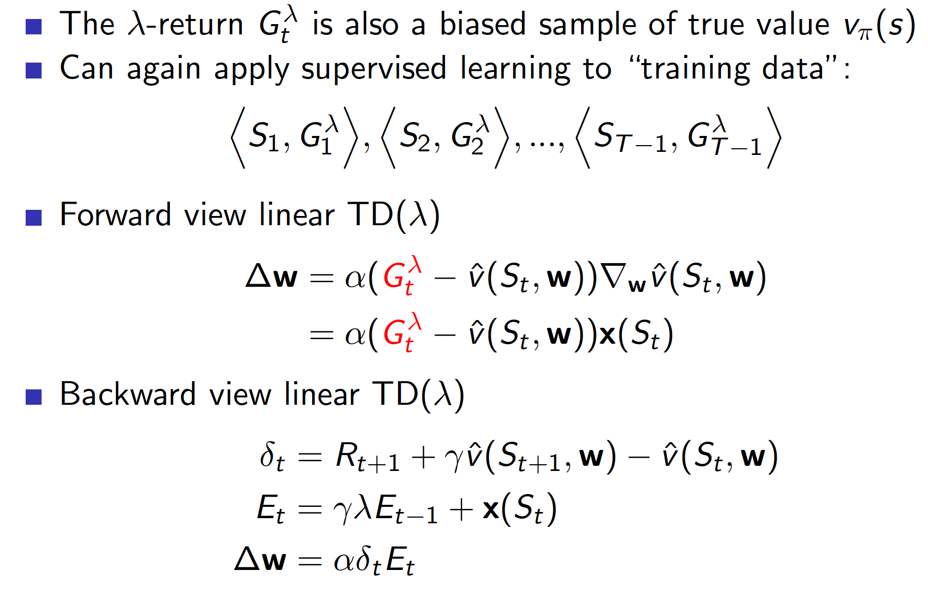
TD($\lambda$) with Function Value Approximation

TD($\lambda$) is implemented in a similar way to TD(0) and MC (see above).

Convergence of Algorithms

The summary below provides information on convergence of different algorithms. Ticks mean that convergence is guaranteed. Crosses mean that the algorithm may not converge.

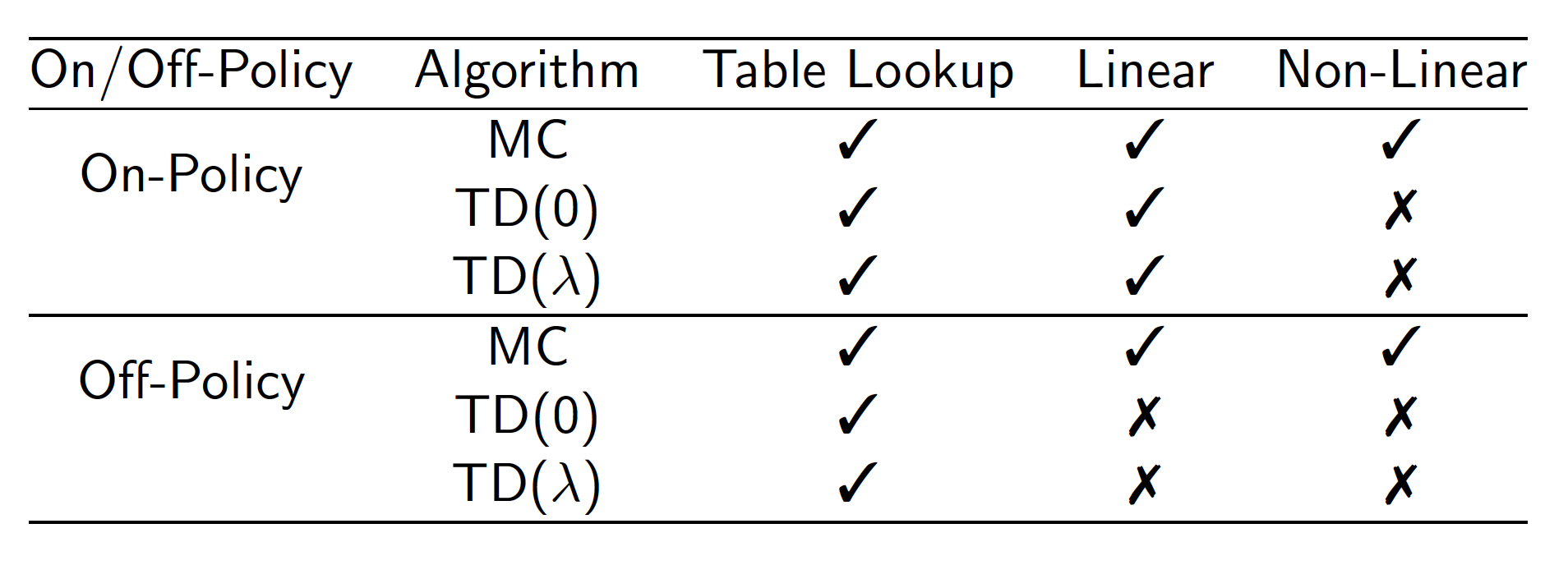
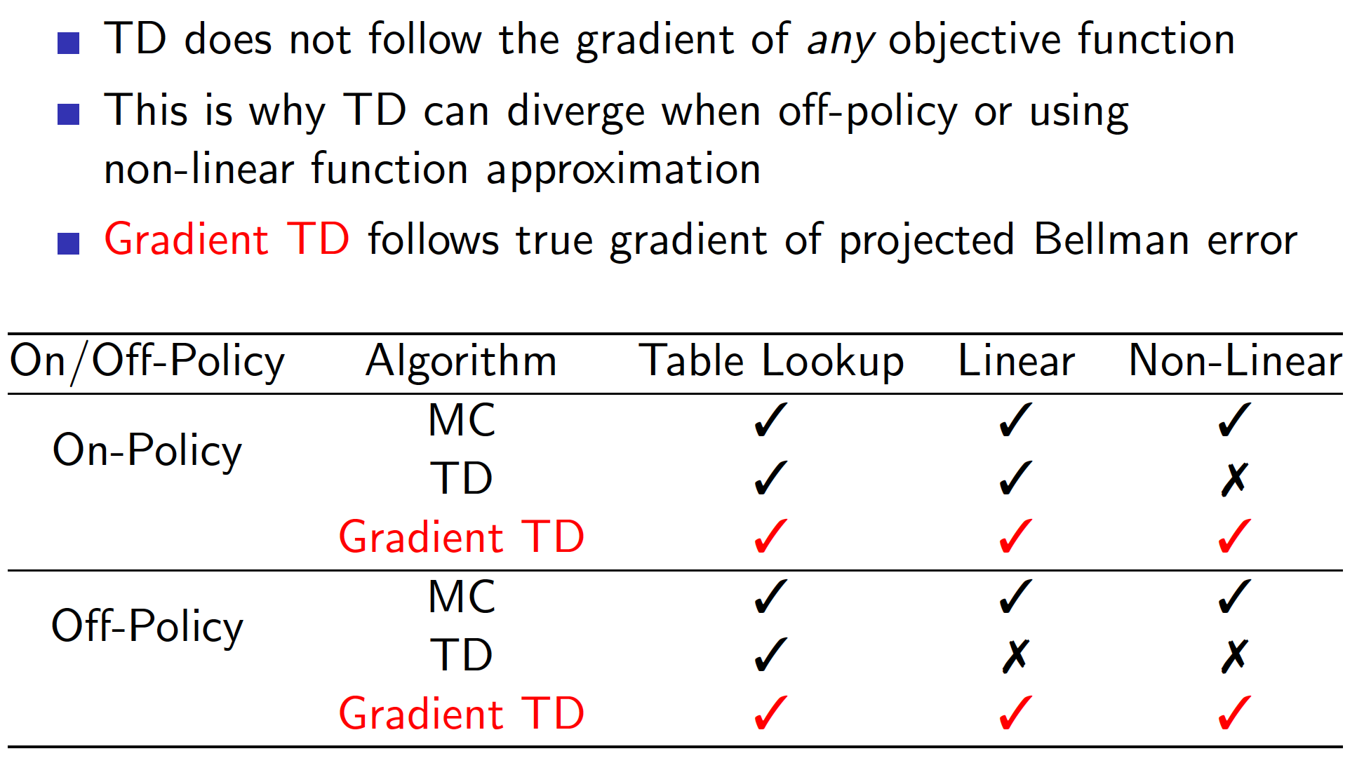
There is an updated version of TD algorithm called Gradient Temporal-Difference Learning. It adds a correction term and, as a result, the algorithm converges.

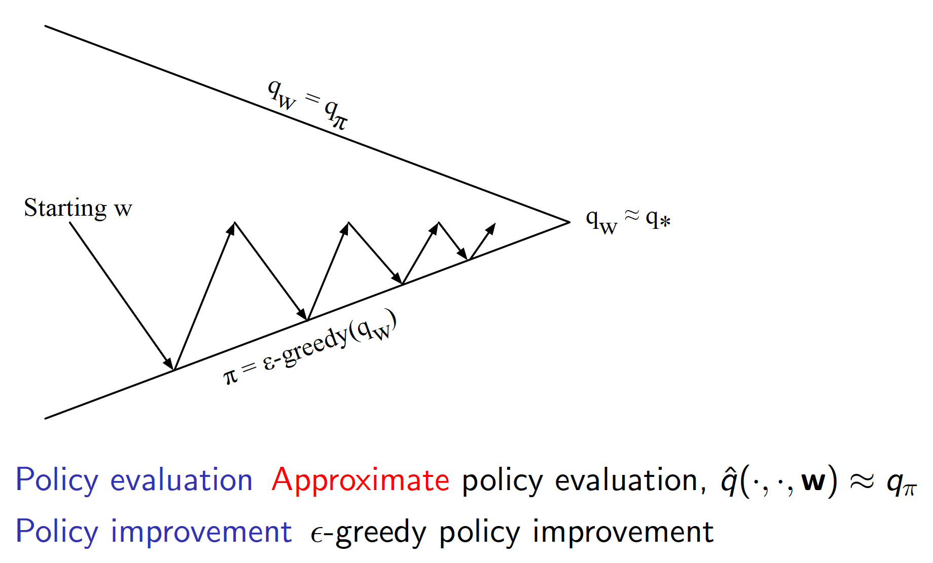
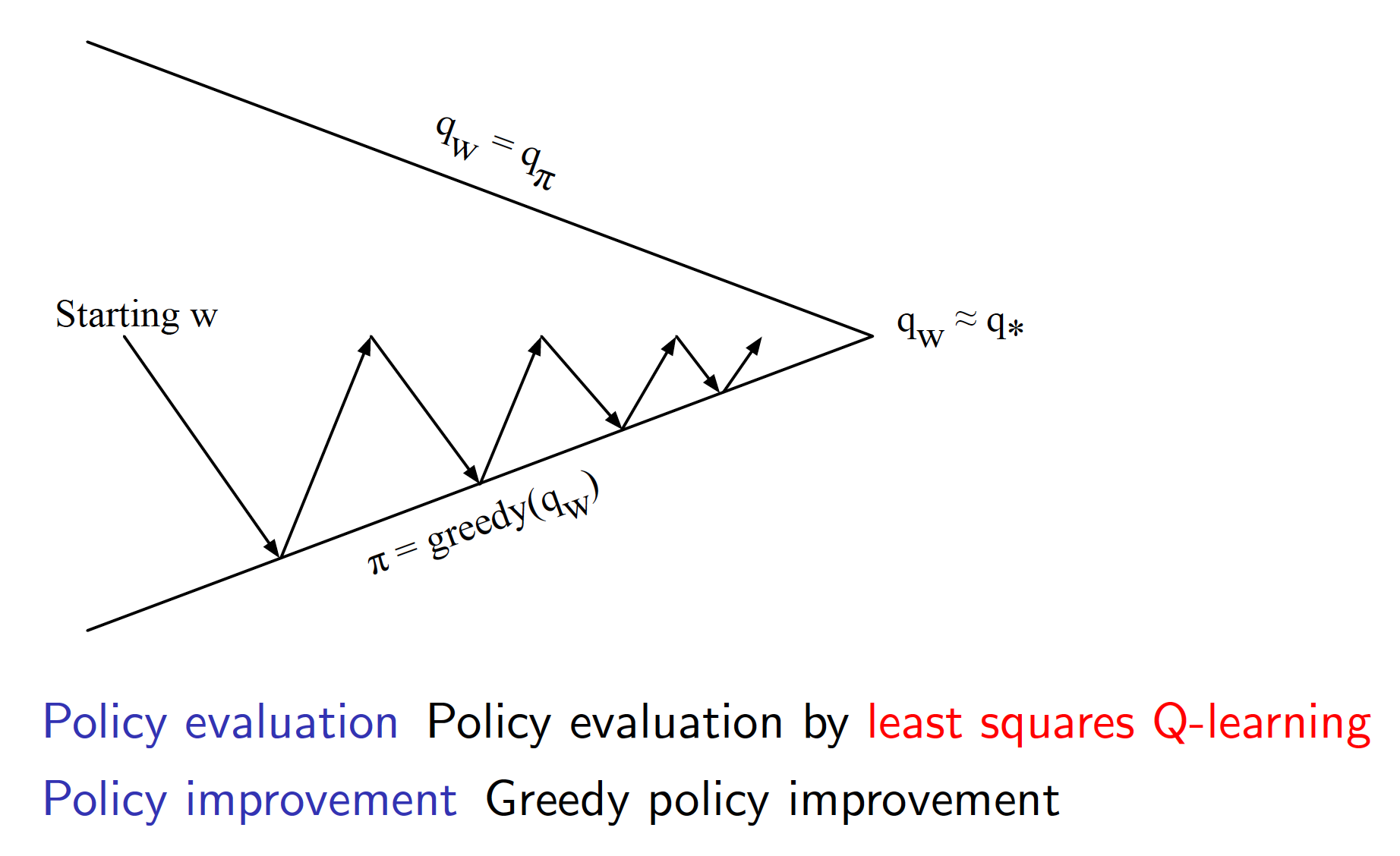
Control with Function Value Approximation

We will approach the problem of control utilizing the idea of the generalized policy iteration. Note that we are using values of state-action pairs instead of state values for control. This ideas have been explored in previous lectures already.

As usual, we first want to find a suitable function approximator for our Q-value function. Once we have decided on that, we can use SGD to fit our function approximator to the true state-action pair values (in practice, we do not know the true state-action values. We are showing it to give an idea).

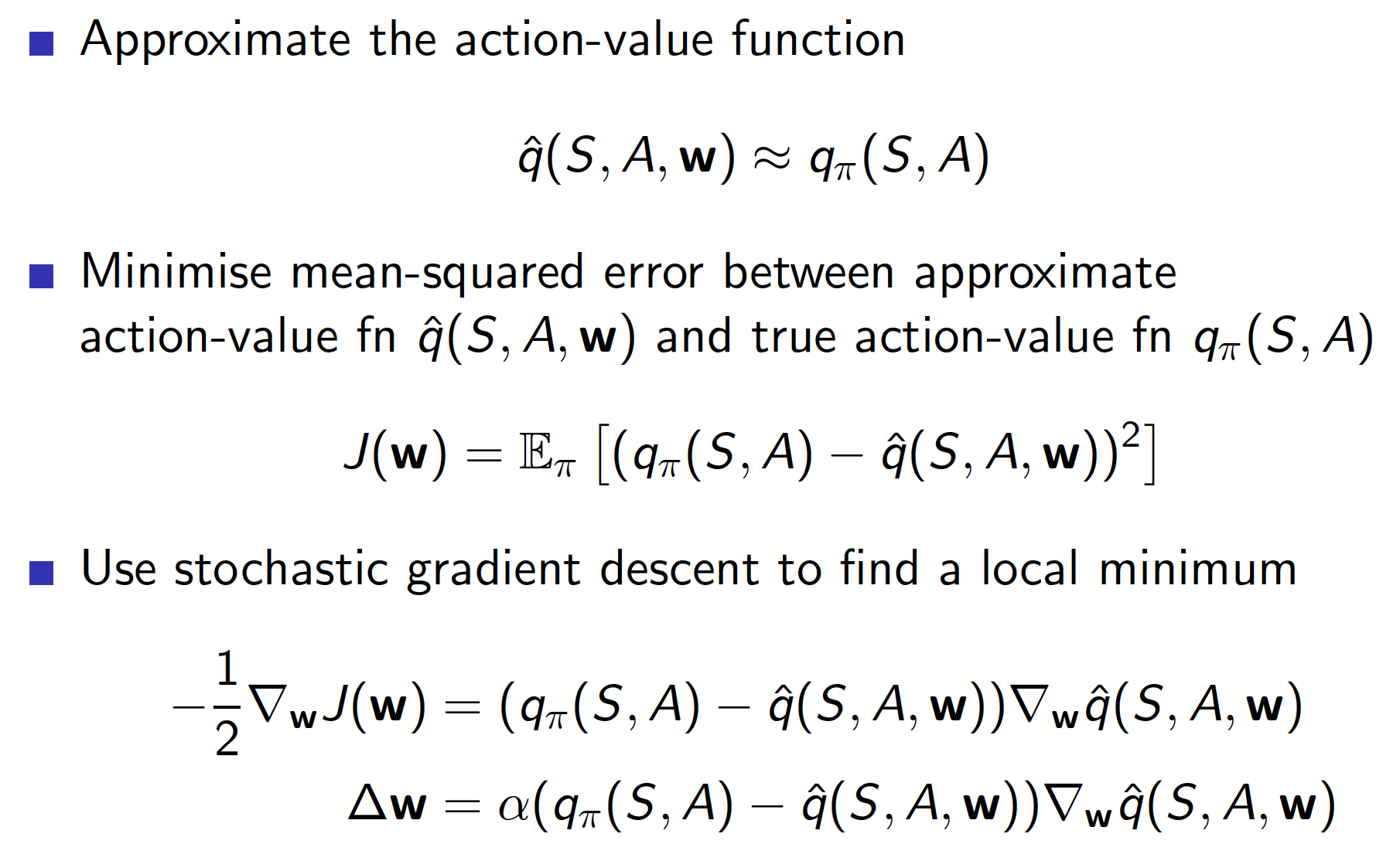
Below we show an example of a linear function approximator, i.e. each state-action pair’s value is represented by a linear combination of suitable features.

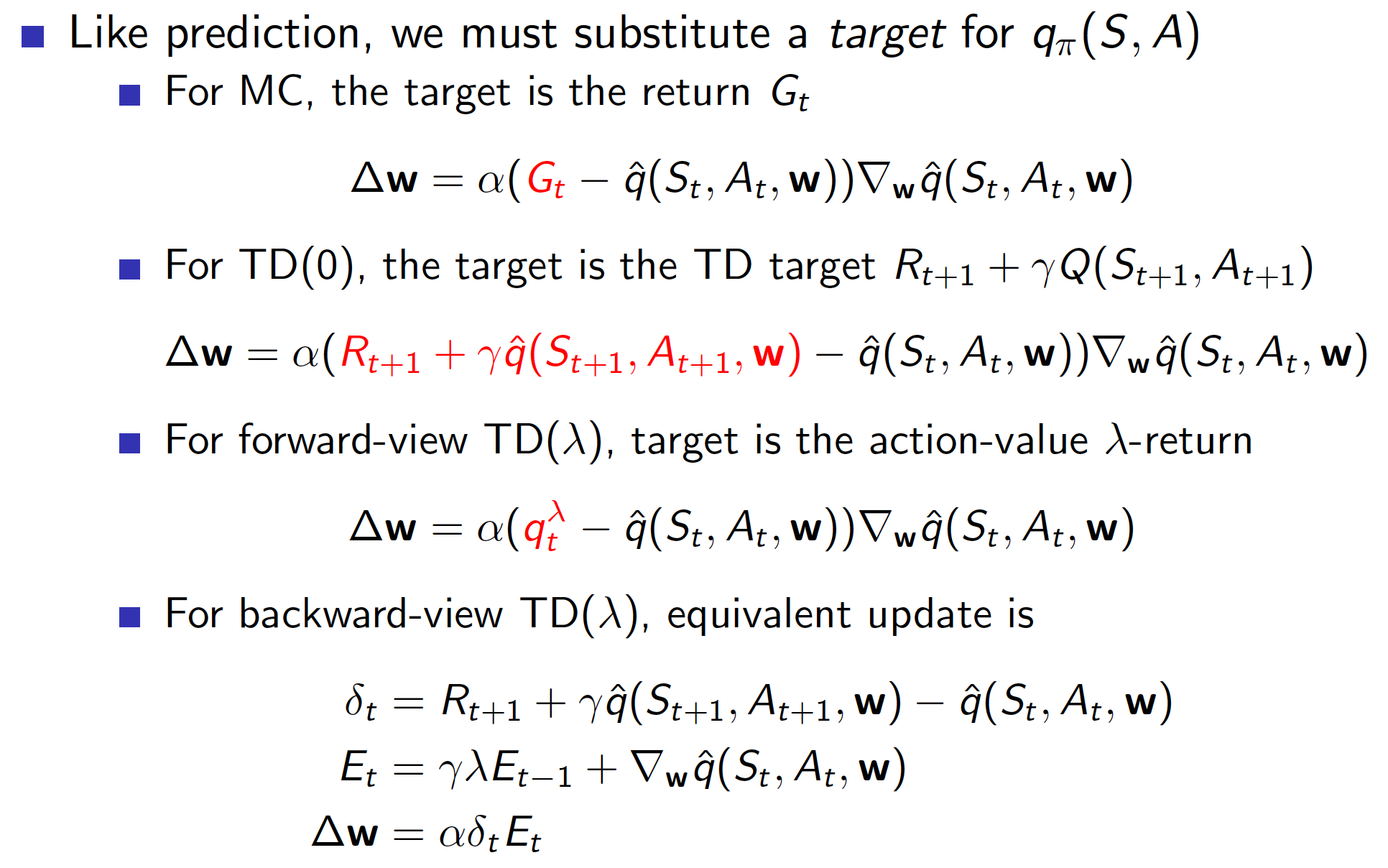
Now, since we do not the true values of state-action pairs, we will use instead our MC, TD and TD($\lambda$) targets.

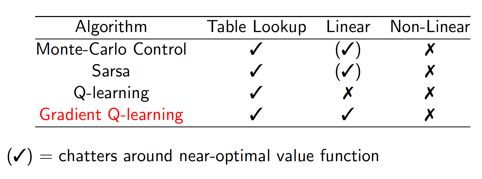
The table below shows the results on convergence of different control algorithms.

Batch Methods

The problems with the approaches that we discussed up to now is that they are not sample-efficient. In other words, once we have updated our value function in the direction of our MC / TD / TD($\lambda$) target, we discard this experience. What we could do instead is collect our experience in a dataset and then learn from that dataset. This is known as experience replay.

For example, Deep Q-learning (DQN) works as follows.

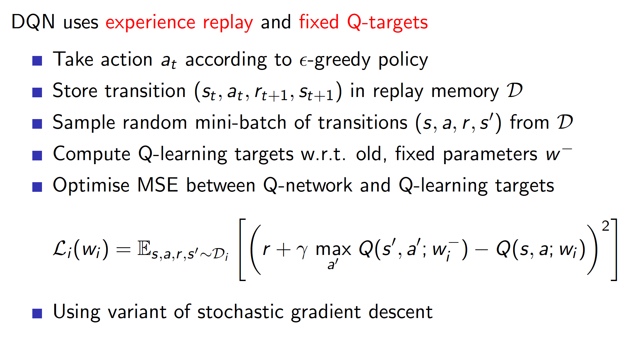
We mentioned previously that SARSA and some other TD methods may diverge. However, this is not the case for DQN, i.e. it is stable (the two reasons for stability are highlighted in red in the above diagram). The first reason is the use of experience replay which “decorrelates” the trajectories, the consecutive samples that we get from interacting with the environment. The second reason is the use of fixed Q-targets. This means that we interact with the environment using an old set of parameters $w^-$ and collect all the observations, rewards and TD targets. We then update the approximator using this experience. If we do not do this, we are effectively updating the parameters of our function approximator that further affect our targets, i.e. there is a circular reasoning.

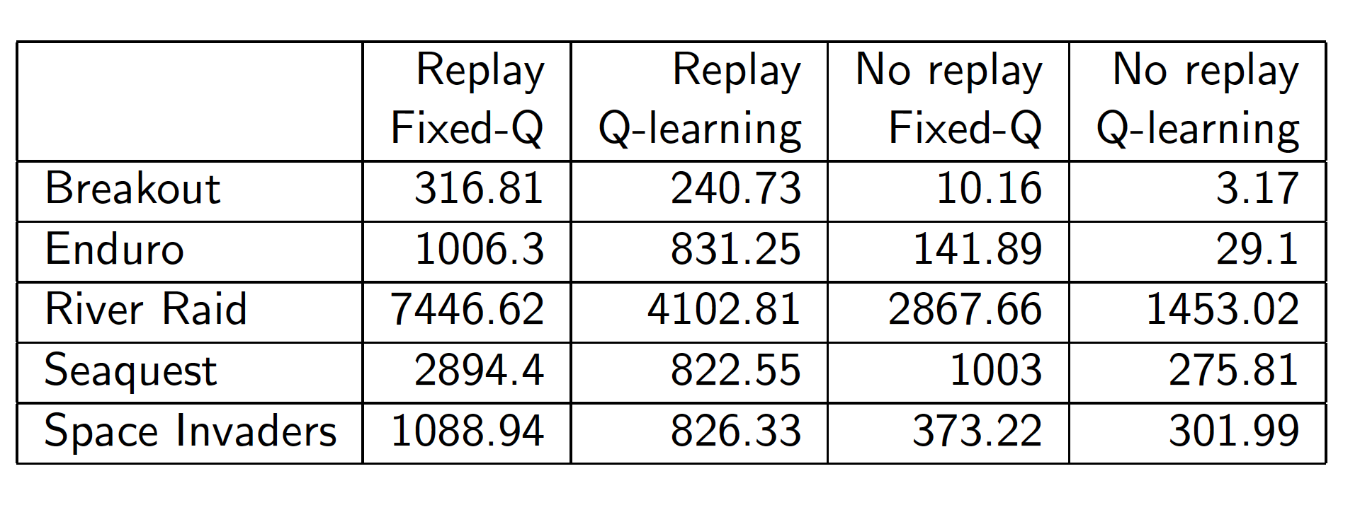
As the diagram below shows, there are benefits of using both of the ideas of experience replay and fixed Q-targets as applied to some of the Atari games.

Linear Least Squares Prediction (Evaluation)

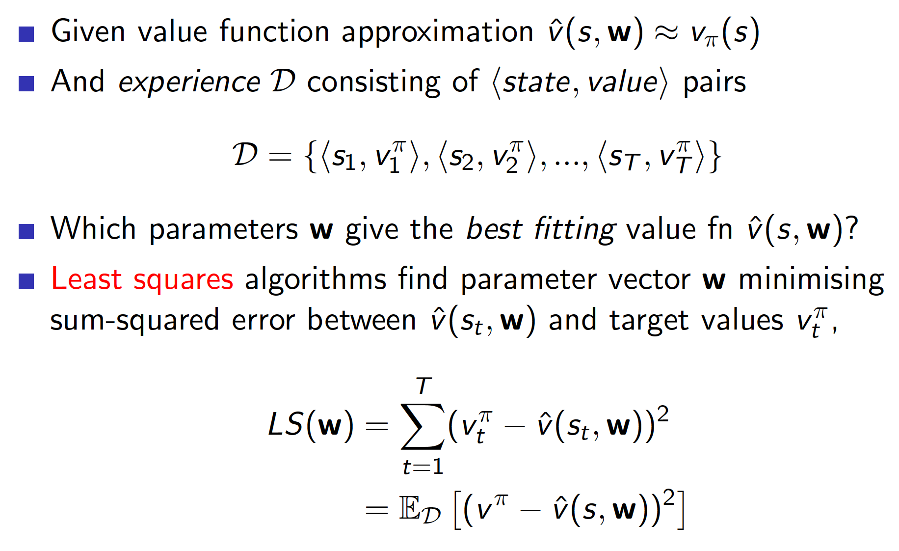
There is a quicker way to evaluate our policy if we use a linear function approximator and make use of experience replay. In other words, we can obtain the least squares solution directly. At the point of minimum squared error, $w^*$, we should have

\[\begin{equation*} E_{D}\left[\Delta w\right] = 0. \end{equation*}\]

This means that the expected change in the parameters of our linear function approximator at the minimum is zero. Expanding the above, we obtain

\[\begin{align*} \alpha \sum_{t=1}^T x(s_t)\left(v_{t}^{\pi} - x(s_t)^Tw\right) &= 0 \\ \alpha \sum_{t=1}^T x(s_t)v_{t}^{\pi} &= \alpha \sum_{t=1}^T x(s_t)x(s_t)^T w \\ w &= \left(\sum_{t=1}^T x(s_t)x(s_t)^T\right)^{-1}\sum_{t=1}^T x(s_t)v_{t}^{\pi}. \end{align*}\]

As usual, our derivation was based on the assumption that we know the true values of our value function, $v_t^{\pi}$. In practice, we use MC, TD and TD($\lambda$) targets.

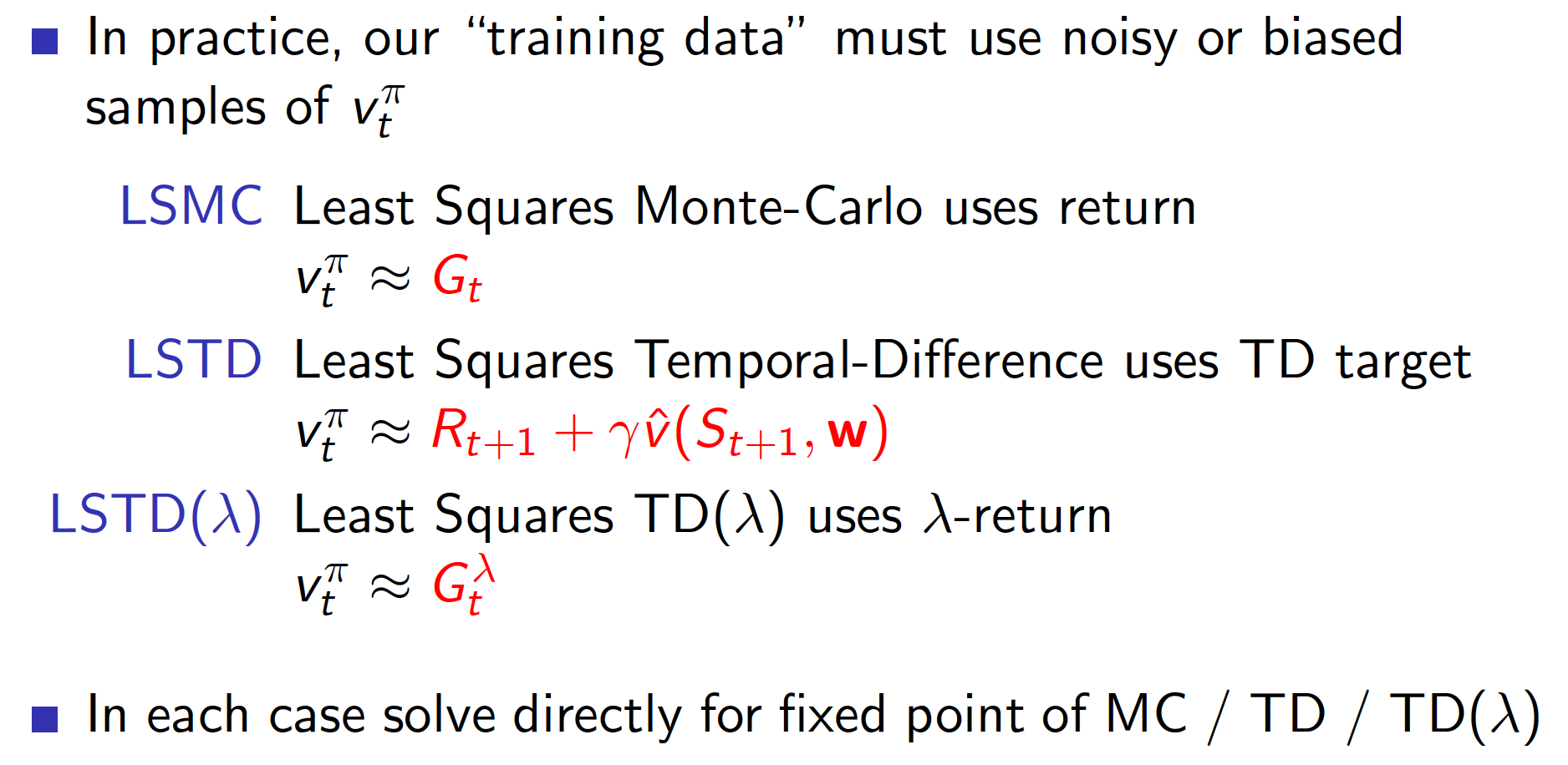
The optimal weights can then be found as

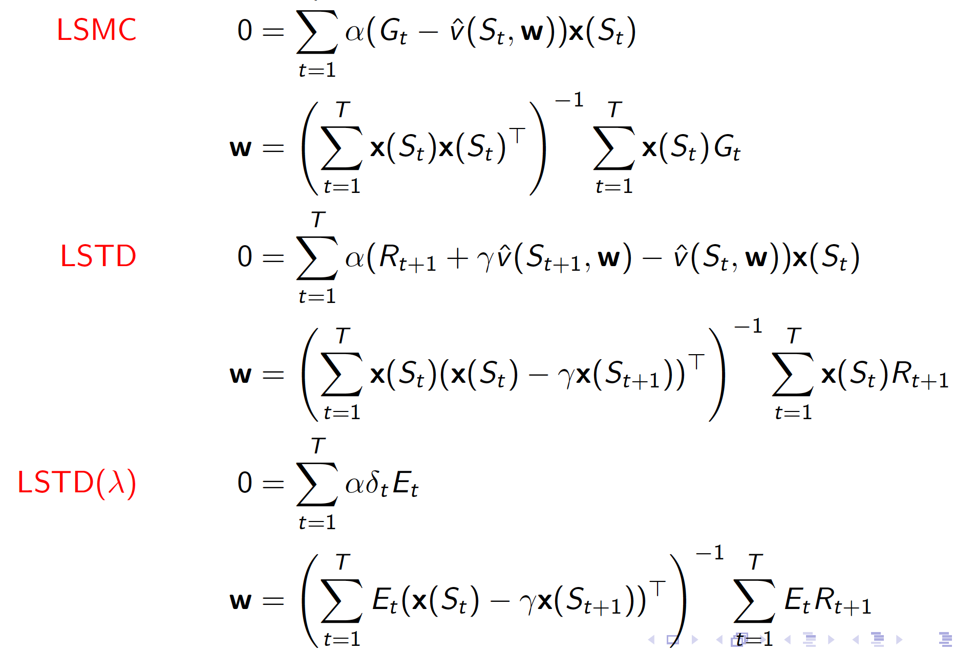
Linear Least Squares Control

We can use the techniques developed in the previous section to derive the optimal policy. Again, as for other control-type problems, the approach is based on generalized policy iteration. But this time we use linear least squares approach to evaluate our policy at each iteration.

More information about linear least squares control can be found in the slides.

Policy Gradient Methods

Policy Gradient (PG) methods are a class of popular RL methods. These methods optimize the policy directly (we do not work with value functions). Value-based approaches that we considered before approximate the true value or action-value functions. Then the policy was generated directly from the approximated value functions. For example, $\epsilon$-greedy policy with respect to some action-value function. PG methods, on the other hand, directly parametrize the policy, i.e.

\[\begin{equation*} \pi_{\theta}(s,a) = P\left[a|s, \theta \right]. \end{equation*}\]

In other words, we directly control the probabilities over actions.

The following diagram shows the distinction between value- and policy-based RL methods.

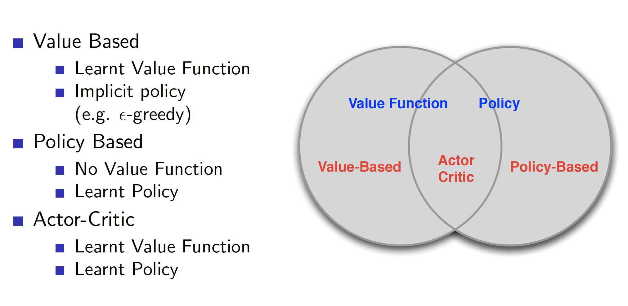
There are certain advantages associated with PG methods:

• better convergence properties (you are guaranteed to at least get to a local optimum)
• effective in high-dimensional or continuous actions spaces. This is the number one reason for using PG methods. When we have a continuous action space, it may become infeasible to pick the best action using value-based methods.
• can learn stochastic policies

Some of the disadvantages are:

• typically converge to a local optimum rather than a global optimum
• evaluating a policy is typically inefficient and high variance

As we can see, learning stochastic policies is an advantage of PG methods. Let us discuss it in more detail. When we use value-based methods, our optimal policy is usually to act greedily with respect to the evaluated policy, i.e. we pick the action than maximizes our value (expected discounted sum of future rewards). This leads to a deterministic policy - we always pick the same action in the same state. However, there may be environments/problems where stochastic policies are favorable. As the first example, consider a game of rock-paper-scissors. The optimal policy is to behave uniformly at random (Nash equilibrium). Any deterministic policy can be easily exploited by an opponent. A second example consists of environments with where the Markov property does not hold. For example, in partially observable environments. Equivalently, we can only use features that give us a limited view of the state of the environment. Consider the following environment:

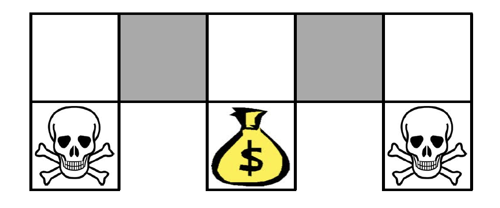
Obviously, our aim is to get to the treasure. At the same time, we do not want to get to the death cells. Assume further that our feature vector $\phi(s,a)$ is of the following form: for all N, S, E, W,

\[\begin{equation*} \phi(s,a) = I(\text{wall to N}, a = \text{move E}). \end{equation*}\]

In other words, for each cell and for each action consisting of N, S, E, W, a given feature tells us if there is a wall in one of the four directions and whether the action is allowed. In total, for each state and action pair, there feature vector would consist of four binary elements. It is not difficult to see that, according to these features, the two gray cells on the above diagram would be considered the same (they both do not have walls to the East and West, they both have walls to the North and South. Finally, the same actions are allowed in both cells). This is known as state aliasing. It follows that any deterministic policy will always choose the same action in both cells (either go West all the time or go East all the time) even though this is clearly not optimal.

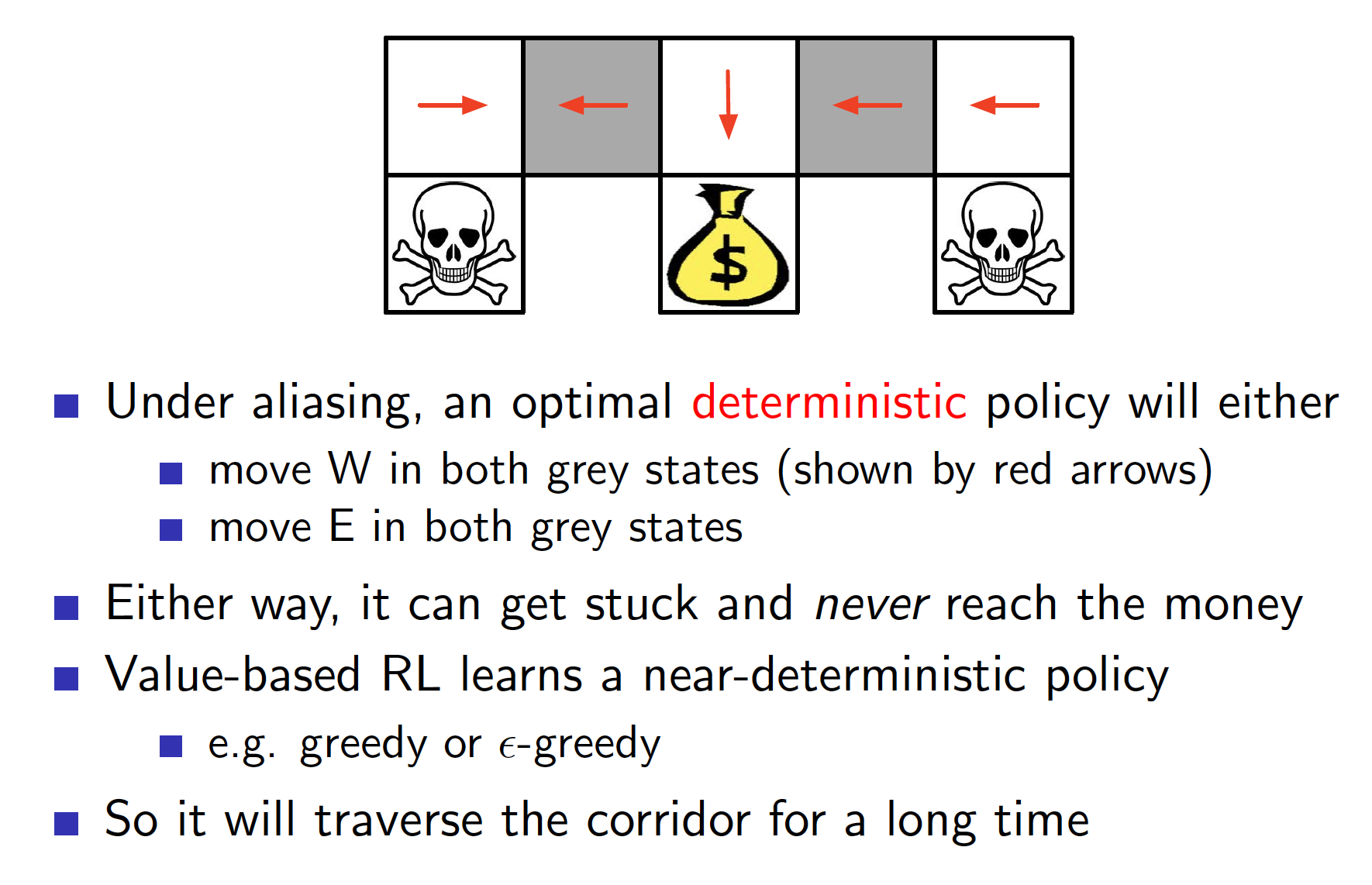
A stochastic policy, which moves either West or East in both of the gray cells, would be optimal in this case.

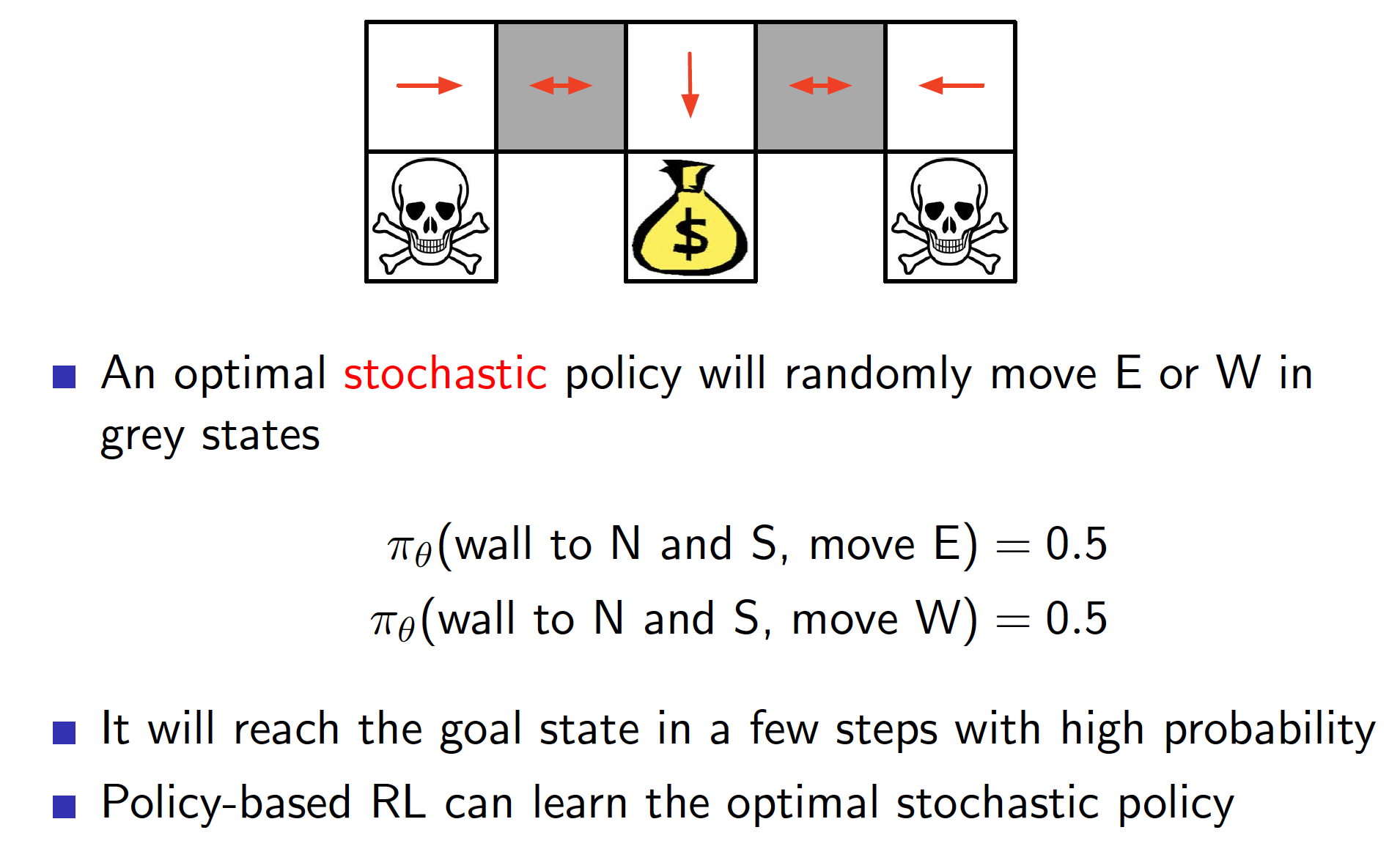
In summary, if we have a perfect state representation, then there will be an optimal deterministic policy. If, however, we have state aliasing, or partial observability, or features that we use give us a limited view of the world, then it can be optimal to use a stochastic policy, i.e. PG methods may do better than value-based methods.

Policy Objective Functions

Before we can talk about policy optimization, we need to specify what our objective is. There are three common options depending on the type of environment:

1. In episodic environments, we can use the start value. We want to maximize the sum of future discounted rewards that our agent expects to get when he starts in state $s_1$ and follows policy $\pi$. This idea works due to the assumption that our agent always starts an episode in the same state or there is a fixed distribution over the starting states.

\[\begin{equation*} J_1(\theta) = V^{\pi_\theta}(s_1) = E_{\pi_\theta}(v_1). \end{equation*}\]

1. In continuing environments, we can use average value.

\[\begin{equation*} J_{avV} = \sum_{s}d^{\pi_\theta}(s)V^{\pi_\theta}(s), \end{equation*}\]

where $d^{\pi_\theta}$ is stationary distribution of Markov chain for $\pi_\theta$ (recall that for a fixed policy a Markov Decision Process, a sequence of states is a Markov Chain). It represents the probability that we end up in state $s$ if we follow our strategy $\pi$.

1. We could also use average reward per time step which can also be used in continuing environments. This objectives states that there is a fixed probability that we end up in some state $s$ and in that state we may take some action $a$ with probability $\pi_{\theta}(s,a)$ which yield us an immediate reward of $R_s^a$.

\[\begin{equation*} J_{avR} = \sum_{s}d^{\pi_\theta}(s)\sum_{a}\pi_{\theta}(s,a)R_s^a. \end{equation*}\]

As it turns out, whichever one objective we choose, we end up with the same gradient. The three objectives are essentially just rescalings of each other.

Now, our aim is to update the parameters $\theta$ of our policy $\pi_{\theta}$ to maximize one of the objectives $J_1, J_{avV}, J_{avR}$. In other words, we want to change the parameters of our policy function so that the probability of those states $s$ where the total discounted sum of total rewards is highest. We could use gradient-free methods like hill climbing, simplex, genetic algorithms, etc. However, greater efficiency can be achieved when gradient information is available. Thus, we should use gradient descent/ascent, conjugate gradient, quasi-newton, etc.

Policy Gradient

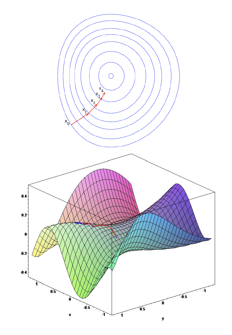
Given an objective function $J(\theta)$ to be maximized, we want to change our parameters $\theta$ in the direction of steepest ascent, i.e.

\[\begin{equation*} \Delta \theta = \alpha \nabla J(\theta), \end{equation*}\]

where $\alpha$ is a step size and $\nabla J(\theta)$ is the gradient of the objective function with respect to $\theta$.

One way to estimate (more correctly, approximate) the gradient is to use a finite difference method. This is a numerical method. Suppose that our parameter vector $\theta$ is n-dimensional. We can then approximate k-th partial derivative of the objective function with respect to $\theta$ by perturbing $\theta$ by a small amount $\epsilon$ in k-th dimension

\[\begin{equation*} \frac{\partial J(\theta)}{\partial \theta_k} = \frac{J(\theta + \epsilon u_k) - J(\theta)}{\epsilon}, \end{equation*}\]

where $u_k$ is unit vector with 1 in k-th component and 0 elsewhere. This requires n evaluations for an n-dimensional parameter vector. Overall, the approach is noisy and inefficient. However, the advantage is that this approach works for arbitrary policies even when they are not differentiable.

Score Function

Of course, estimating the gradient of the objective function using the method of finite differences is very inefficient. Instead, we want to estimate the gradient analytically. Assume that the policy function $\pi_{\theta}(a,s)$ is differentiable with respect to the parameters $\theta$. Then,

\[\begin{align*} \nabla_{\theta} \pi_{\theta}(a,s) &= \pi_{\theta}(a,s) \frac{\nabla_{\theta} \pi_{\theta}(a,s)}{\pi_{\theta}(a,s)} \\ &= \pi_{\theta}(a,s) \nabla_{\theta} \ln \pi_{\theta}(a,s), \end{align*}\]

where we used a useful identity $\nabla_{x} \ln f(x) = \frac{\nabla_x f(x)}{f(x)}$. Function $\nabla_x \ln f(x)$ is known as the score function.

As a first example, consider a softmax policy. According to softmax policy, the probability of taking any action $a$ is state $s$ is given by

\[\pi_{\theta}(a,s) = \frac{e^{\phi(s,a)^T \theta}}{\sum_{a \in A} e^{\phi(s,a)^T \theta}},\]

where $\phi(s,a)$ is a vector of features. The corresponding score function is derived as follows

\[\begin{align*} \nabla_{\theta} \ln \pi_{\theta}(s,a) &= \nabla_{\theta} \ln \left(\frac{e^{\phi(s,a)^T \theta}}{\sum_{a \in A} e^{\phi(s,a)^T \theta}} \right)\\ &= \phi(s,a) - \nabla_{\theta} \ln \left(\sum_{a \in A} e^{\phi(s,a)^T \theta}\right) \\ &= \phi(s,a) - \frac{\nabla_{\theta} \sum_{a \in A} e^{\phi(s,a)^T \theta}}{\sum_{a \in A} e^{\phi(s,a) \theta}} \\ &= \phi(s,a) - \frac{\sum_{a \in A}e^{\phi(s,a)^T \theta} \phi(s,a)}{\sum_{a \in A} e^{\phi(s,a)^T \theta}} \\ &= \phi(s,a) - \sum_{a \in A} \phi(s,a) \pi_{\theta}(s,a) \\ &= \phi(s,a) - E_{\pi_{\theta}}\left[\phi(s,\cdot)\right]. \end{align*}\]

When we work in an environment with a continuous action space, a Gaussian policy might be used. According to this policy, in any given state $s$, an action is sampled from a Gaussian distribution with mean $\mu(s) = \phi(s)^T \theta$ and variance $\sigma^2$. In other words, the probability any any action $a$ in state $s$ is taken is equal to

\[\begin{align*} \pi_{\theta}(a,s) = \frac{1}{\sigma \sqrt{2\pi}} e^{-\frac{1}{2}\left(\frac{a - \phi(s)^T \theta}{\sigma}\right)^2} \end{align*}\]

Note that variance $\sigma^2$ can be fixed or also parametrized. The corresponding score function is obtained as

\[\begin{align*} \nabla_{\theta} \ln \pi_{\theta}(a,s) &= \nabla_{\theta} \left( \ln \frac{1}{\sigma \sqrt{2\pi}} -\frac{1}{2}\left(\frac{a - \phi(s)^T \theta}{\sigma}\right)^2 \right) \\ &= \nabla_{\theta} \left( -\frac{1}{2\sigma^2} \left(a^2 - 2a\phi(s)^T\theta + \left(\phi(s)^T\right)^2\theta^2 \right) \right) \\ &= \frac{\phi(s)}{2\sigma^2} \nabla_{\theta} \left(2a\theta - \phi(s)^T \theta^2\right) \\ &= \frac{\phi(s)}{2\sigma^2} \left(2a - 2\phi(s)^T\theta \right) \\ &= \frac{\phi(s) \left(a - \mu(s)\right)}{\sigma^2}. \end{align*}\]

Consider a one-step MDP where we start in some state $s \sim d(s)$. An episode terminates after a single step with a reward $r = R_{s,a}$. The objective function is the expected reward, i.e.

\[\begin{align*} J(\theta) &= E_{\pi_{\theta}}\left[r\right] \\ &= \sum_{s \in S} d(s) \sum_{a \in A}\pi_{\theta}(s,a)R_{s,a}. \end{align*}\]

Taking the gradient,

\[\begin{align*} \nabla_{\theta} J(\theta) &= \nabla_{\theta} \sum_{s \in S} d(s) \sum_{a \in A} \pi_{\theta}(s,a)R_{s,a} \\ &= \sum_{s \in S} d(s) \sum_{a \in A} \nabla_{\theta} \pi_{\theta}(s,a) R_{s,a} \\ &= \sum_{s \in S} d(s) \sum_{a \in A} \pi_{\theta}(s,a) \nabla_{\theta} \ln \pi_{\theta}(s,a) R_{s,a} \\ &= E_{\pi_\theta}\left[\nabla_{\theta} \ln \pi_{\theta}(s,a) r\right] \end{align*}\]

What the above expression says is that to optimize our policy, we should move in the direction of the score function times the reward.

Policy Gradient Theorem

The policy gradient theorem generalizes the likelihood ratio approach to multi-step MDPs. We replace the instantaneous reward with the long-term value $Q_{\pi}(s,a)$.

Theorem For any differentiable policy $\pi_{\theta}(s,a)$ and for any of the policy objective functions $J = J_1$, $J_{avR}$ or $\frac{1}{1 - \gamma}J_{avV}$, the policy gradient is

\[\begin{equation} \nabla J(\theta) = E_{\pi_\theta}\left[\nabla_{\theta} \ln \pi_{\theta}(s,a) Q_{\pi_\theta}(s,a) \right] \end{equation}\]

REINFORCE

REINFORCE is one of the simplest algorithms that makes use of the policy gradient theorem. Here we use the realized return $v_t$ as an unbiased estimated of $Q_{\pi_\theta}(s_t, a_t)$. The algorithm itself is

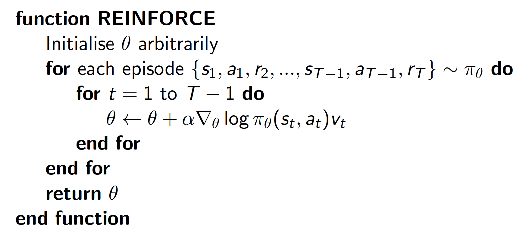
Actor-Critic Methods

As we know from previous lectures, Monte-Carlo returns are unbiased estimates of the true returns but they are high variance estimates. Instead, we could use the ideas developed in the previous lecture and complement our policy function (actor) with state-action value approximator (critic). This combination gives rise to actor-critic approaches of RL:

• critic updates the parameters $w$ of state-action value function $Q_{w}(s,a)$
• actor updates the parameters $\theta$ of the policy function $\pi_{\theta}(s,a)$

Effectively, our critic guides our actor and tells him how to adjust its parameters to maximize the objective function. Actor-critic algorithms follow an approximate policy gradient

\[\begin{align*} \nabla_{\theta} J(\theta) \approx E_{\pi_\theta}\left[\nabla_{\theta}\ln \pi_{\theta}(s,a)Q_w(s,a)\right] \\ \Delta \theta = \alpha \nabla_{\theta}\ln \pi_{\theta}(s,a) Q_w(s,a). \end{align*}\]

Note that we can use MC, TD or TD($\lambda$) method to evaluate our current action-value function.

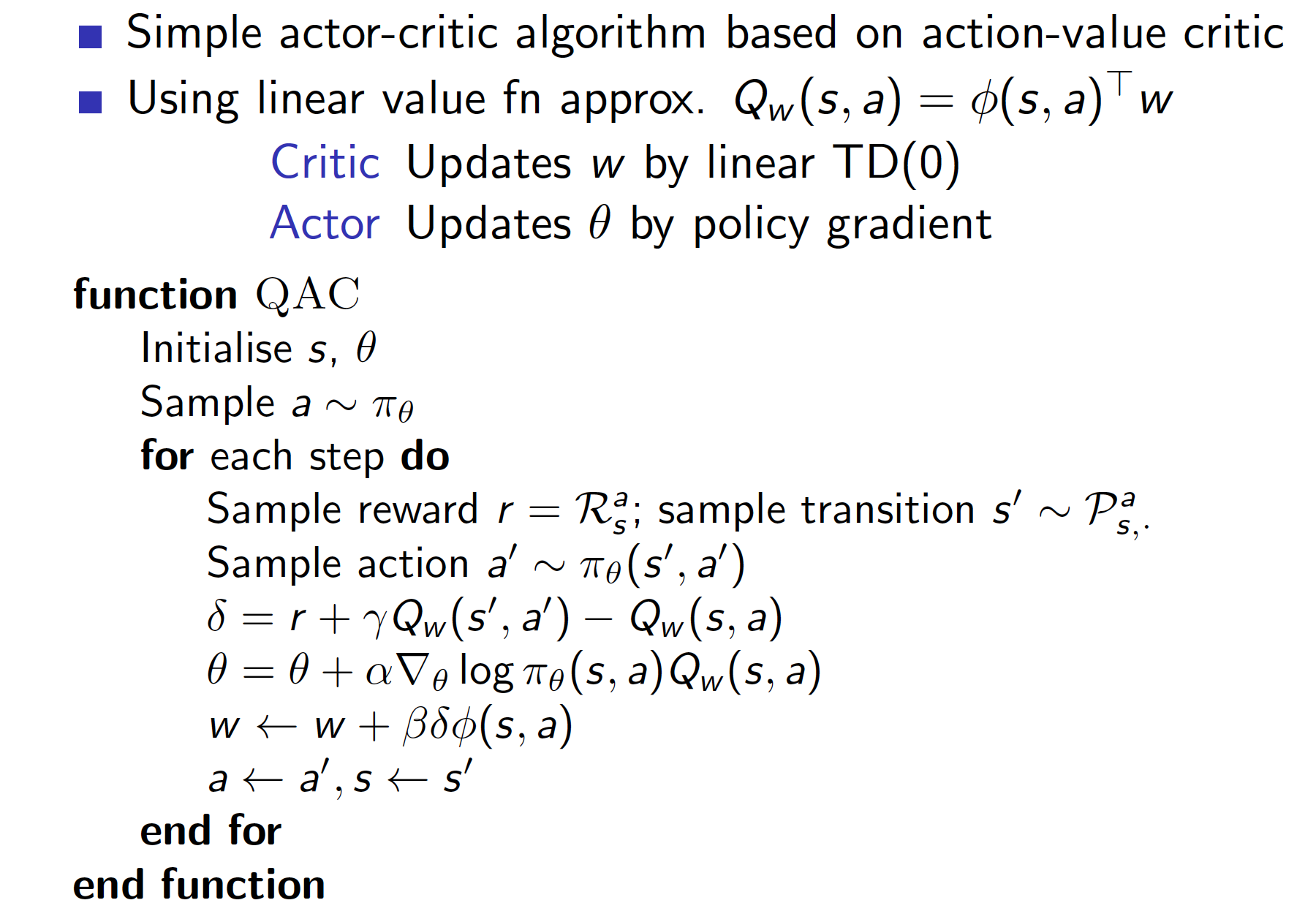
While we reduce the variance of the one hand, we may introduce bias on the other hand when using a critic. And biased gradient may not find the right solution. However, if we are careful in choosing our value function approximator, then we can avoid introducing any bias. The theorem below provides the requirements.

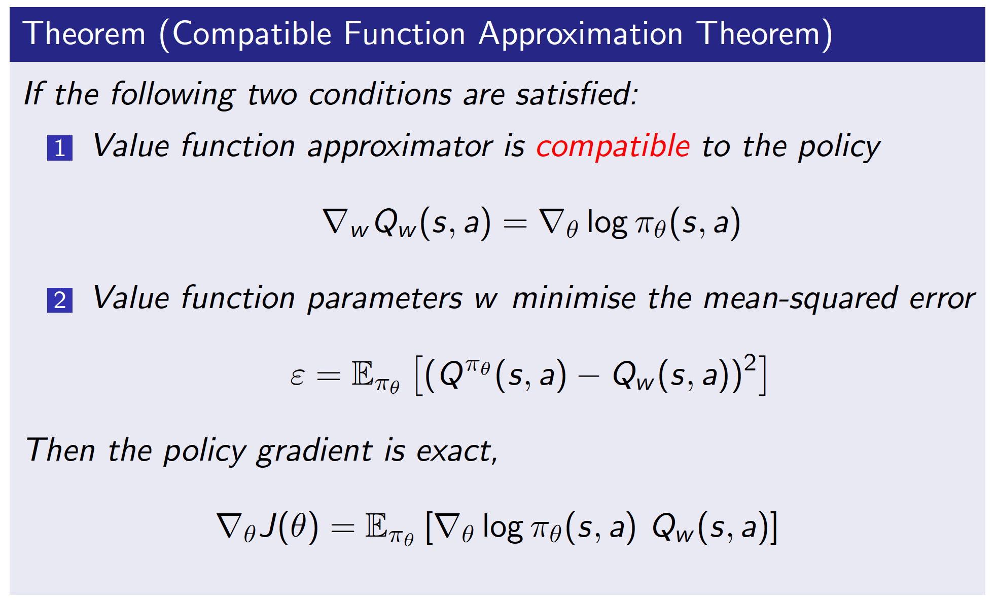
Advantage Function

Another way to reduce the variance is to subtract some baseline function $B(s)$ from the policy gradient. Recall that the gradient is estimated as

\[\begin{equation*} \nabla_{\theta}J(\theta) = E_{\pi_\theta}\left[\nabla_{\theta}\ln \pi_{\theta}(s,a) Q_{\pi_\theta}(s,a)\right]. \end{equation*}\]

Observe that

\[\begin{align} E_{\pi_\theta}\left[\nabla_{\theta}\ln \pi_{\theta}(s,a)B(s)\right] &= \sum_{s \in S}d_{\pi_\theta}(s) \sum_{a \in A} \pi_{\theta}(s,a) \nabla_{\theta} \ln \pi_{\theta}(s,a) B(s) \label{eq:advantage}\\ &= \sum_{s \in S}d_{\pi_\theta}(s) \sum_{a \in A} \pi_{\theta}(s,a) \frac{\nabla_{\theta} \pi_{\theta}(s,a)}{\pi_{\theta}(s,a)} B(s) \nonumber \\ &= \sum_{s \in S}d_{\pi_\theta}(s) B(s) \nabla_{\theta} \sum_{a\in A} \pi_{\theta}(s,a) \nonumber \\ &= \sum_{s \in S}d_{\pi_\theta}(s) B(s) \nabla_{\theta} \sum_{a\in A} 1 \nonumber \\ &= 0 \nonumber, \end{align}\]

where we used the useful identity $\nabla_{\theta}\ln \pi_{\theta}(s,a) = \frac{\nabla_{\theta}\pi_{\theta}(s,a)}{\pi_{\theta}(s,a)}$ and the fact that the gradient of a constant is equal to 0. Since the quantity as per Equation ($\ref{eq:advantage}$) is equal to 0, we can safely add or subtract it from the equation of a gradient of the objective function, i.e.

\[\begin{align*} \nabla_{\theta}J(\theta) &= E_{\pi_\theta}\left[\nabla_{\theta}\ln \pi_{\theta}(s,a) Q_{\pi_\theta}(s,a)\right] - E_{\pi_\theta}\left[\nabla_{\theta}\ln \pi_{\theta}(s,a)B(s)\right] \\ &= E_{\pi_\theta}\left[\nabla_{\theta}\ln \pi_{\theta}(s,a) \left(Q_{\pi_\theta}(s,a) - B(s)\right)\right] \\ &= E_{\pi_\theta}\left[\nabla_{\theta}\ln \pi_{\theta}(s,a) A_{\pi_\theta}(s,a)\right], \end{align*}\]

where $A_{\pi_{\theta}}$ is known as advantage function. Intuitively, the advantage function tells us how much better it is to take action $a$ in state $s$ as compared to the value of being in state $s$, i.e. how much more reward is expected to be achieved by taking action $a$ than what would be otherwise expected in state $s$. A common choice of baseline function is the state-value function $V_{\pi_{\theta}}(s)$.

Estimating the Advantage Function

We understand how using the advantage function can help us reduce the variance. How do we estimate the advantage function? One way is to make our critic learn both the state-value and action-value functions. For example, let $V_{v}(s)$ be state-value function approximator parametrized by $v$ and $Q_{w}(s,a)$ be action-value function approximator parametrized by $w$. The advantage function $A(s,a)$ can then be approximated as

\[\begin{equation*} A(s,a) = Q_w(s,a) - V_v(s). \end{equation*}\]

The value functions can be “learned” as usual, i.e. using TD, MC and TD($\lambda$) learning approaches covered in previous lectures.

There is, however, a better way to estimate/approximate the advantage function. The idea here is that for the true value function $V_{\pi_{\theta}}(s)$, the TD error is an unbiased estimated of the advantage function. Recall that the TD error $\delta_{\pi_{\theta}}$ for the true value function $V_{\pi_{\theta}}$ is

\[\begin{equation*} \delta_{\pi_{\theta}} = r + \gamma V_{\pi_{\theta}}(s') - V_{\pi_{\theta}}(s). \end{equation*}\]

The expectation of the TD error is

\[\begin{align*} E_{\pi_{\theta}}\left[\delta_{\pi_{\theta}}\right] &= E_{\pi_{\theta}}\left[r + \gamma V_{\pi_{\theta}}(s') - V_{\pi_{\theta}}(s)|s,a\right] \\ &= E_{\pi_{\theta}}\left[r + \gamma V_{\pi_{\theta}}(s')|s,a\right] - V_{\pi_{\theta}}(s) \\ &= Q_{\pi_{\theta}}(s,a) - V_{\pi_{\theta}}(s) \\ &= A_{\pi_{\theta}}(s,a). \end{align*}\]

This means that we can use the TD error to estimate the gradient of the objective function, i.e.

\[\begin{equation*} \nabla_{\theta}J(\theta) = E_{\pi_{\theta}}\left[\nabla_{\theta}\ln \pi_{\theta}(s,a) \delta_{\pi_{\theta}}\right]. \end{equation*}\]

In practice, since we are using function approximators, we would have

\[\begin{equation*} \delta_{v} = r + \gamma V_{v}(s') - V_v(s). \end{equation*}\]

This approach is more efficient as it requires a single set of parameters $v$ and a single value function to be estimated.

Critic can estimate the value function $V_{\theta}(s)$ from many different targets and from different time-scales.

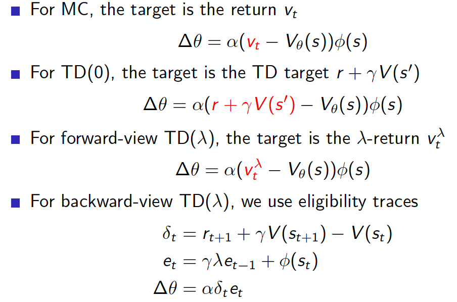
Similarly, the policy gradient can also be estimated at many different time-scales.

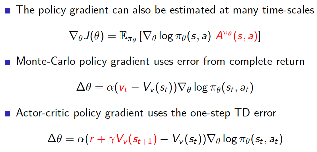
Using eligibility traces,

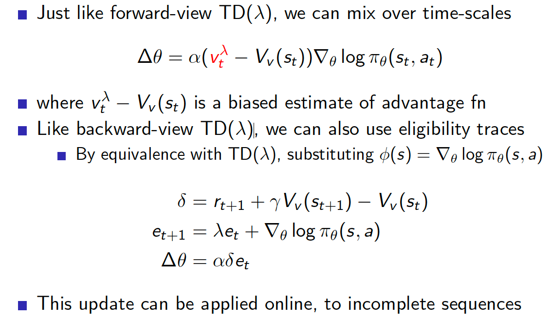
Summary

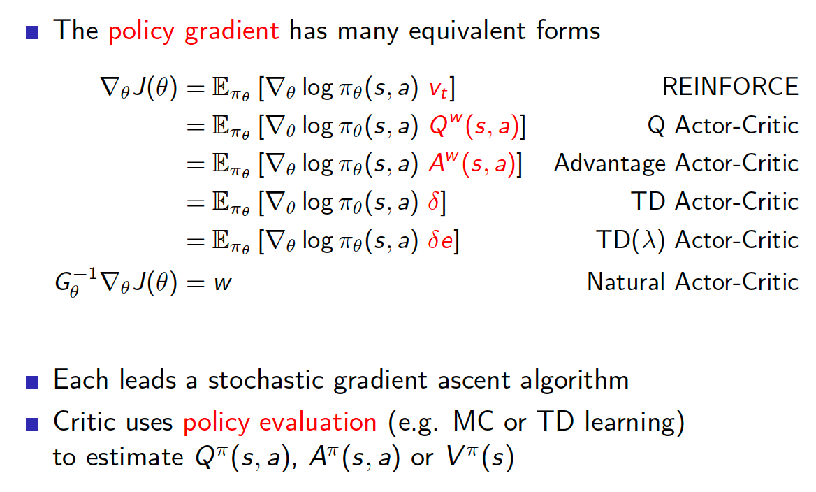
Integrating Learning and Planning

Up to now we studied how an agent can learn a policy or a value function directly from experience. The approaches did not require that we know anything about how the environment operates. The aim of this lecture is to investigate whether our agent can learn the model of the environment from experience, i.e. state-transition probabilities and the rewards. Once we know the model of the environment we can do planning. Planning means that our agent can look ahead to construct a value function or a policy. For example, we could use tree-search methods as in the game of chess.

Recall that in model-free RL our agent directly interacted with the environment, i.e. observed the state of the environment, took actions and received rewards. Schematically this can be represented as follows

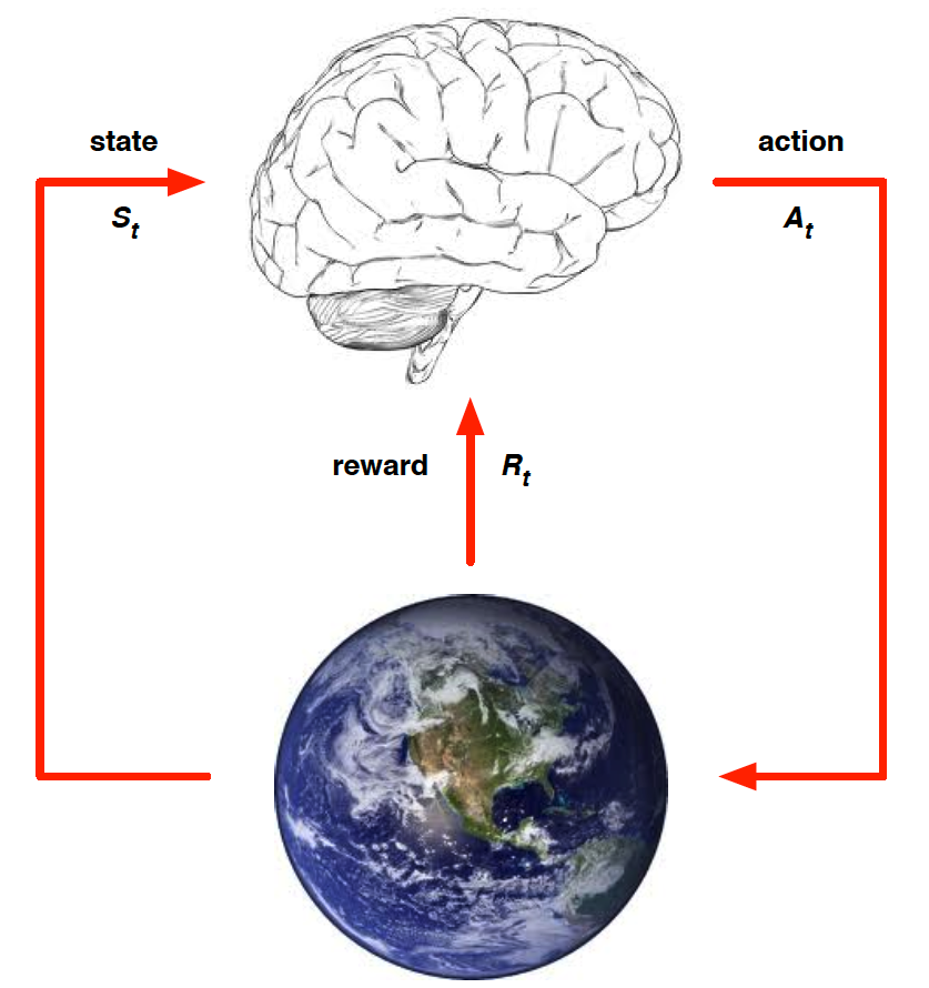
In model-based RL, on the other hand, our agent first learns a “model” of the environment, i.e. some kind of representation of the actual environment, and then engage in planning as explained above.

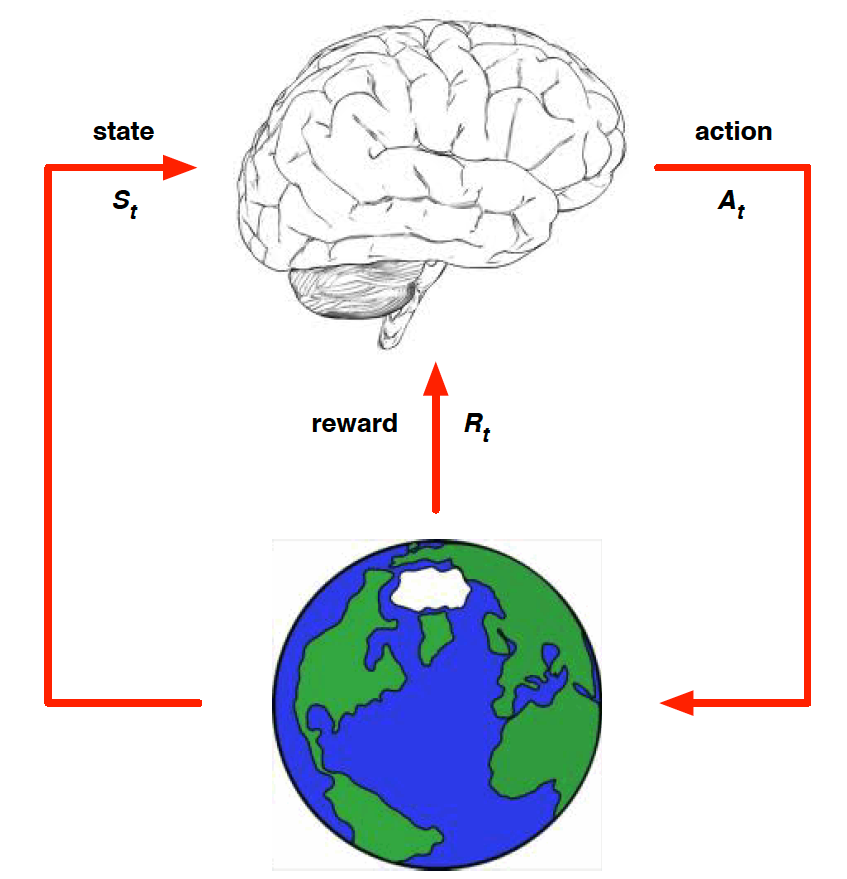
Model-Based RL

Model-based RL cycle is shown on the diagram below.

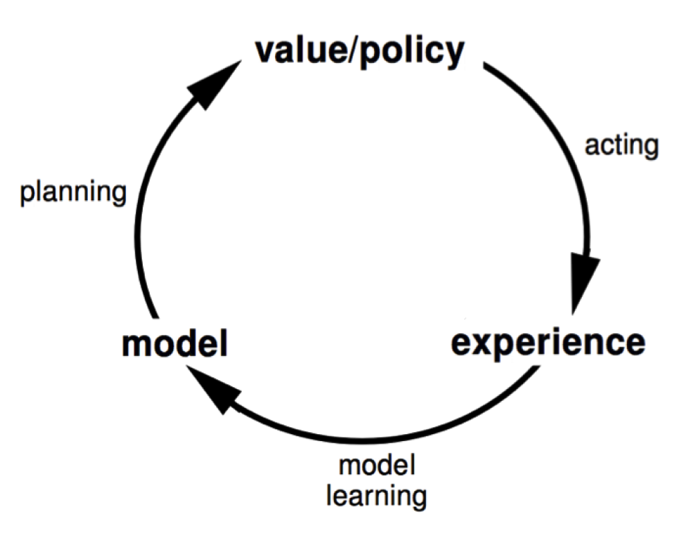
Our agent starts by interacting with the real environment and getting experience. From that experience the agent can construct a model of the environment. By constructing a model we mean constructing an MDP. The model is then used for planning, i.e. looking ahead to estimate the value function or the policy (since learned the model of the environment, we can use dynamic programming techniques for that). The learned policy and/or value function can then be used in the real environment.

There are certain and advantages and disadvantages associated with model-based RL. Some of the advantages include:

• Obviously, model-based RL is very useful in the domains where learning value functions and policies directly from experience is hard. For example, take a game of chess. There are positions where a single bad move can transform a completely winning position to a completely losing one. This means that a very similar input to the model should produce drastically different estimates of the value function. Given that there are so many different positions in chess, it may become very difficult to learn the value function directly from experience. On the other hand, the model of the environment is quite simple - it is just the rules of the game. For example, if you take an action of moving a pawn two cells up, the resulting positions is clearly known. Knowing how the environment works can simplify our search for the value function. In chess, we could use tree-search.
• We can learn the model by using the techniques of supervised learning.
• Can reason about model uncertainty

The main disadvantage of the model-based RL is that we first need to learn a model and only then can construct the value function. This means that there are effectively two sources of approximation error.

What is a Model?

A model $M$ is a representation of an MDP $<S, A, P, R>$ that is parametrized by $\eta$ (for example, a neural network or a table lookup). Let us suppose that we know the state and action spaces. This is a simple case, but in reality these may not be known to us. In this case, a model $M_{\eta} = <P_{\eta}, R_{\eta}>$ represents state transitions $P_{\eta} \approx P$ and rewards $R_{\eta} \approx R$, i.e.

\[\begin{align*} S_{t+1} \sim P_{\eta}\left[S_{t+1}| S_t, A_t\right], \\ R_{t+1} = R_{\eta}\left[R_{t+1}|S_t, A_t\right]. \end{align*}\]

We usually also assume conditional independence between state transitions and rewards, i.e.

\[\begin{equation*} P\left[S_{t+1}, R_{t+1}| S_{t}, R_t\right] = P\left[S_{t+1}|S_t, R_t\right]P\left[R_{t+1}|S_t, R_t\right]. \end{equation*}\]

Some common choices of models include:

• table lookup model
• linear expectation model
• linear Gaussian model
• Gaussian process model
• deep belief network

Model Learning

We want to learn $M_{\eta}$ from experience $<S_1, A_1, R_1, S_2, \cdots., S_T>$. This can be treated as a supervised learning problem. That is,

\[\begin{align*} S_1, A_1 &\rightarrow R_1, S_2 \\ S_2, A_2 &\rightarrow R_2, S_3 \\ &\vdots \\ S_{T-1}, A_{T-1} &\rightarrow R_{T-1}, S_T. \end{align*}\]

In particular, we can use regression analysis, $s,a \rightarrow r$, to learn the reward function. Learning the state-transition function, $s, a \rightarrow s’$, can be treated as density estimation problem. We choose the appropriate loss functions (for example, MSE for regression and KL divergence for density estimation) and find such parameters $\eta$ that minimize the overall loss.

Table Lookup Model

One of the simplest models is the table lookup model. There are two ways to estimate this model. The first one is based on counting. In other words, we start by counting how many times we visited each state and action pair $N(s,a)$. Then,

\[\begin{align*} \hat{P}_{ss'}^{a} &= \frac{1}{N(s,a)}\sum_{t=1}^T I_{\left\{S_t, A_t, S_{t+1}=s,a,s'\right\}}, \\ \hat{R}_s^a &= \frac{1}{N(s,a)} \sum_{t=1}^T I_{\{S_t, A_t = s,a\}}R_t. \end{align*}\]

The other approach is based on memorizing the tuples $<S_t, A_t, R_t, S_{t+1}>$. When we want to sample from this model, we randomly choose $R_t$ and $S_{t+1}$ from those tuples that match $<s,a,\cdot, \cdot>$.

The following example (AB example) demonstrates a model that was learned/constructed using the counting method.

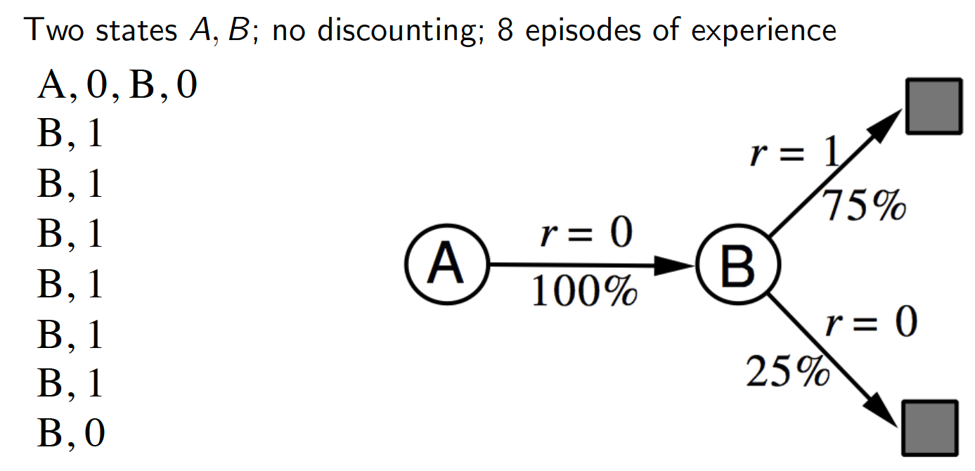
Since we only experienced a single transition from state $A$ to state $B$, the learned probability of transitioning from $A$ to $B$ is 100% (with no corresponding reward). Similarly, 6 out of 8 transitions (75%) from state $B$ resulted in a reward of 1 and the remaining 2 (25%) resulted in no reward.

Planning with a Model

Given a model $M_{\eta}$ of the environment, how do we proceed solving it (meaning solving the MDP $<S, A, P_{\eta}, R_{\eta}>$)? Actually, we can choose any of the planning algorithms:

• value iteration
• policy iteration
• tree search
• etc.

A simple but a very effective approach to planning is to use the model only to generate experience to which we can then apply any of the model-free learning approaches, i.e. MC control, SARSA, Q-learning, etc. So, basically, model-based approaches are reduced to model-free approaches once we have learned the model of the environment. Sample-based approaches to the problem of planning are oftentimes more efficient.

Applying this idea to the AB example introduced above, we may get the following solution to the MDP.

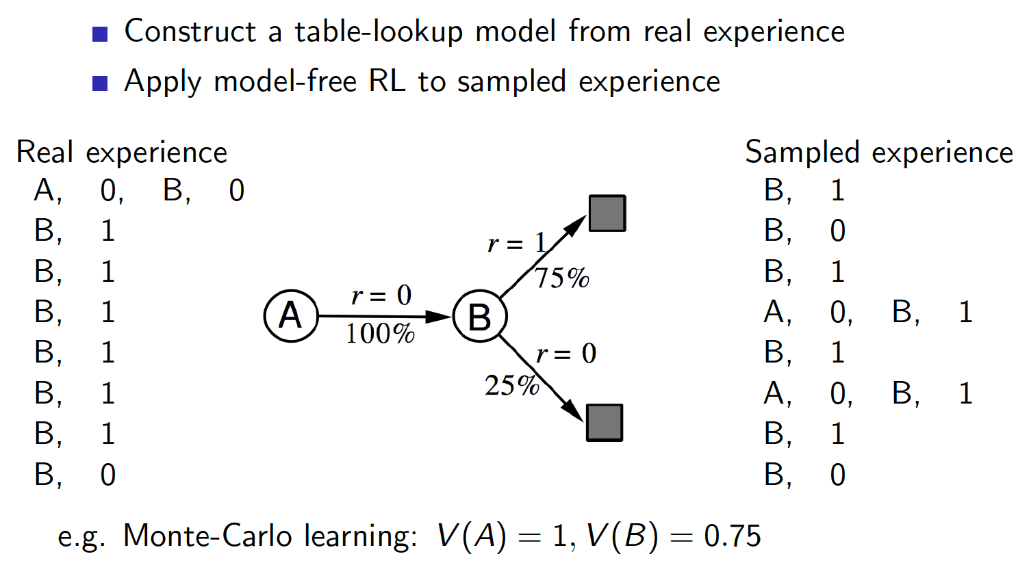
Planning with an Inaccurate Model

Model-based RL is only as good as the estimated model. Of course, if our experience of the real environment is limited, we may not learn a correct model, i.e. $<P_{\eta}, R_{\eta}> \ne <P, R>$. In this case, the planning process will result in a suboptimal policy. The possible solutions include:

• use model-free RL
• reason explicitly about model uncertainly

Integrated Architectures

Integrated architectures are all about combining the best of two worlds - model-free and model-based RL. For these, we are going to use experience generated from two sources: real experience from the true MDP and simulated experience from the learned model (approximate MDP). The approach that learns a value function or a policy using both the real and simulated experience is known as Dyna. The picture below shows the differences between model-free, model-based and Dyna RL approaches.

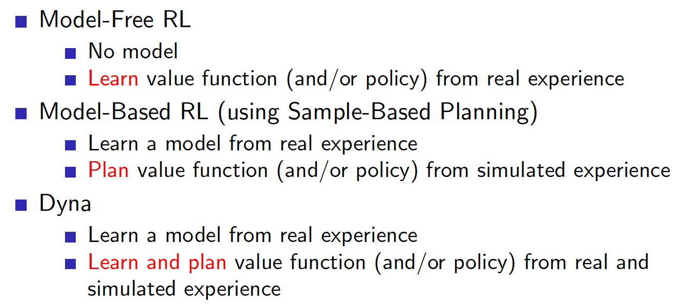
The learning cycle of the Dyna approach is shown below.

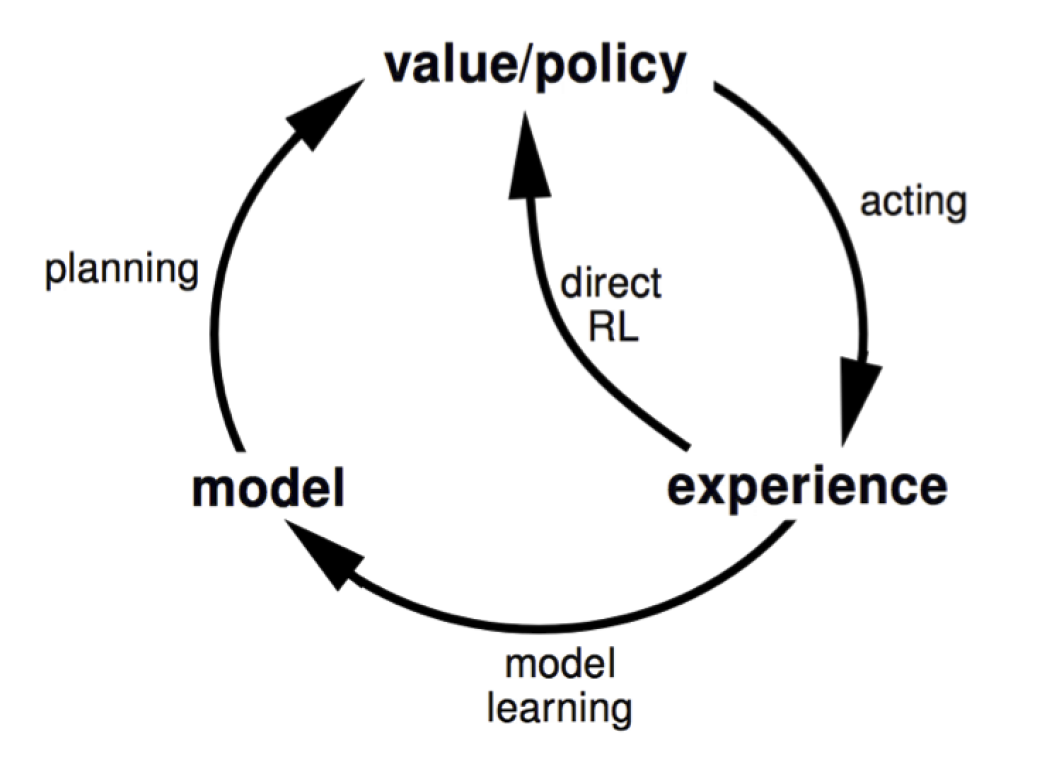
One caveat with using the Dyna approach is that we should be smart about how we combine the two streams of experience. The simplest algorithm is known as Dyna-Q algorithm. It takes the following form.

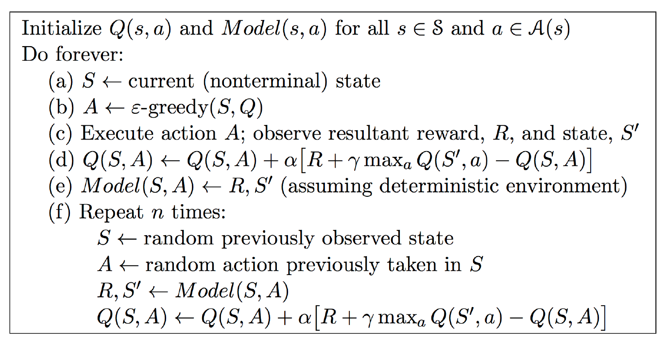
The above algorithm requires a little bit of explanation. First of all, we start by initializing both $Q(s,a) $ and $Model(s,a)$, i.e we do not wait until the model of the environment is fully constructed. Steps $a$ to $d$ are the usual Q-learning steps, i.e. we are learning the action-value function by directly interacting with the environment. Step $e$ is the supervised leaning step that helps us to construct the model of the environment by observing the real experience. Finally, step $f$ is the “thinking loop”. Here our agent “imagines” a possible transition from state $S$ to state $S’$ and a possible reward $R$ from the model of the environment that can then be used in the Q-learning update.

Simulation-Based Search

This part is not about learning a model per se but more about the problem of planning given a model. The key ideas are sampling and forward search.

Forward Search

Forward search algorithms work by building a search tree with the current state $s_t$ at the root. These algorithms select the best action in the current state by using a model of the MDP to look ahead. Effectively, what this means is that there is no need to solve the whole MDP but just a sub-MDP starting from the current state.

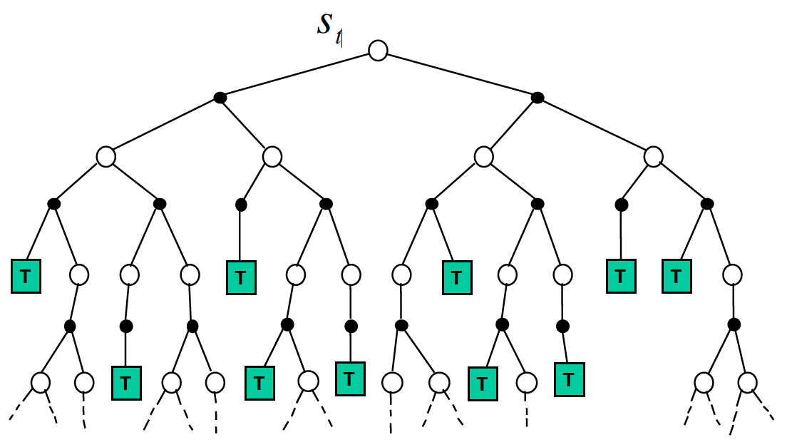
Simulation-Based Search

This is a forward search paradigm that uses sample-based planning. It consists of simulating episodes of experience starting from the current state with the learned model and applying the model-free RL techniques to these simulated episodes to choose the best action in the current state.

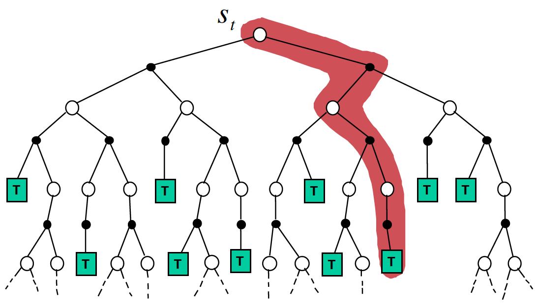
We start by simulating $k$ episodes of experience from the current state with the model:

\[\begin{align*} \left\{s_t^1, A_t^1, R_t^1, S_{t+1}^1, \cdots, S_T^1\right\} &\sim M_{\eta} \\ \left\{s_t^2, A_t^2, R_t^2, S_{t+1}^2, \cdots, S_T^2\right\} &\sim M_{\eta} \\ & \vdots \\ \left\{s_t^k, A_t^k, R_t^k, S_{t+1}^k, \cdots, S_T^k\right\} &\sim M_{\eta} \end{align*}\]

We proceed by applying model-free RL to the simulated episodes:

• Monte-Carlo control gives rise to Monte-Carlo search
• SARSA gives rise to TD search
• etc.

Simple Monte-Carlo Search

Suppose we have estimated a model $M_{\eta}$. Let us now simulate experience from this model using some simulation policy $\pi$ (simulation policy is just the way we are simulating experience from our agent’s “imagination”). In particular, for each available action $a$ in the current state $s_t$, simulate $k$ episodes of experience

\[\begin{align*} \left\{s_t^1, A_t^1, R_t^1, S_{t+1}^1, \cdots, S_T^1\right\} &\sim M_{\eta}, \pi \\ \left\{s_t^2, A_t^2, R_t^2, S_{t+1}^2, \cdots, S_T^2\right\} &\sim M_{\eta}, \pi \\ & \vdots \\ \left\{s_t^k, A_t^k, R_t^k, S_{t+1}^k, \cdots, S_T^k\right\} &\sim M_{\eta}, \pi \end{align*}\]

Now evaluate each action as the mean return, i.e.

\[\begin{equation*} Q(s_t, a) = \frac{1}{k}\sum_{i=1}^{k}G_t. \end{equation*}\]

Then choose that action $a$ at the current state $s_t$ in the “real world” that yields the highest average reward

\[\begin{equation*} a_t = \underset{a\in A}{argmax}Q(s_t, a). \end{equation*}\]

For example, in the game of Go, a simple MC search could look something like this.

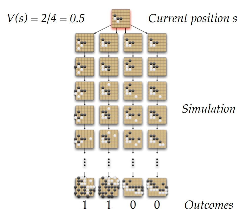
Monte-Carlo Tree Search

Monte-Carlo tree search is a state of the art search algorithm that allowed computers to achieve human-level performance in Go. Similar to the simple MC search, we have a model $M_{\eta}$ and we find ourselves in some root state $s_t$. We simulate $k$ episodes or trajectories of experience using some simulation policy $\pi$.

\[\begin{align*} \left\{s_t^1, A_t^1, R_t^1, S_{t+1}^1, \cdots, S_T^1\right\} &\sim M_{\eta}, \pi \\ \left\{s_t^2, A_t^2, R_t^2, S_{t+1}^2, \cdots, S_T^2\right\} &\sim M_{\eta}, \pi \\ & \vdots \\ \left\{s_t^k, A_t^k, R_t^k, S_{t+1}^k, \cdots, S_T^k\right\} &\sim M_{\eta}, \pi \end{align*}\]

However, the difference with the simple MC search is that we do not just evaluate the action at the root, i.e. at the current state. Instead, we are building a search tree for all the state and action pairs that we visited in the simulated experience. Effectively, we are building something like

The estimate of a value associated with taking any action $a$ in any visited state $s$ is

\[\begin{equation*} Q(s,a) = \frac{1}{N(s,a)}\sum_{i=1}^{k}\sum_{u=t}^T I_{\left\{S_u, A_u = s,a\right\}}G_u. \end{equation*}\]

Having finished the search, select that action with the highest value in the search tree.

\[\begin{equation*} a_t = \underset{a\in A}{argmax}Q(s,a). \end{equation*}\]

The nice thing about MC tree search is that as we generate more experience (trajectories), our simulation policy improves, i.e. actions with higher Q-values are more likely to be chosen in the simulation than actions with lower Q-values. If we are in a situation where we have never been before, we can continue using the default policy of, say, picking actions uniformly at random (until we have constructed a search tree).

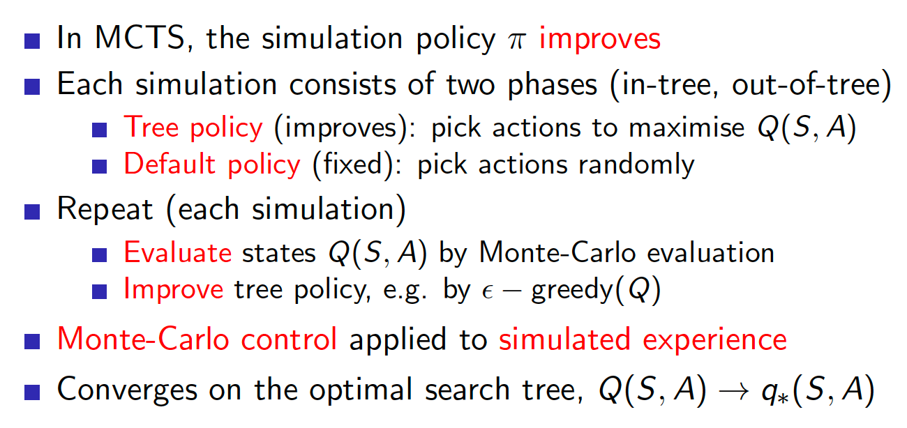
Let us discuss an example of how this algorithm is applied to the game of Go. We start in the current state and simulate a single trajectory that resulted in a win, i.e. a reward of 1. We add the current state to the tree and assign a value of 1 to it (note that we only add the current state to the tree even though we visited multiple states during a trajectory).

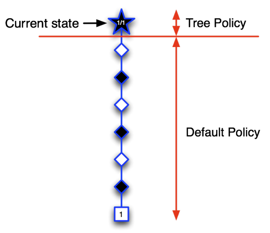
We continue to simulate trajectories from the current state. The second trajectory resulted in the loss and a reward of 0. So we add the second state to the search tree and update the value of the current state to 0.5.

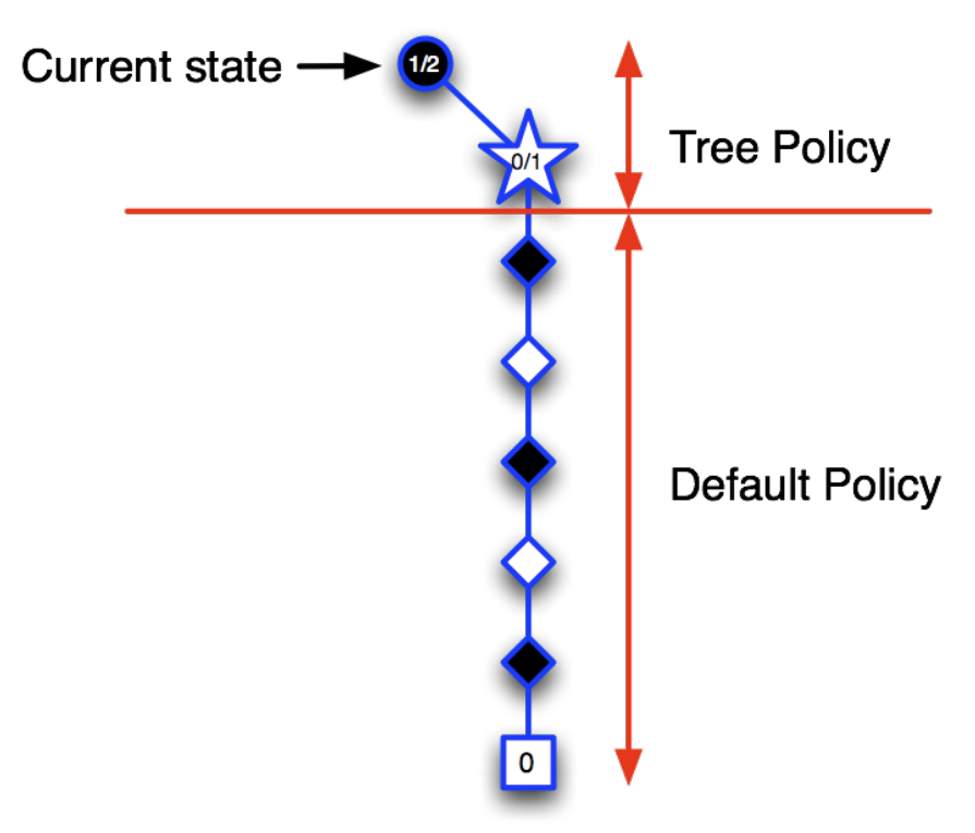
Now, we can utilize the tree policy to guide our choices of actions to generate further trajectories. Since the previous action resulted in a lost game, we generate a new trajectory by taking a different action and adding it to the search tree (we also update the value of the root state).

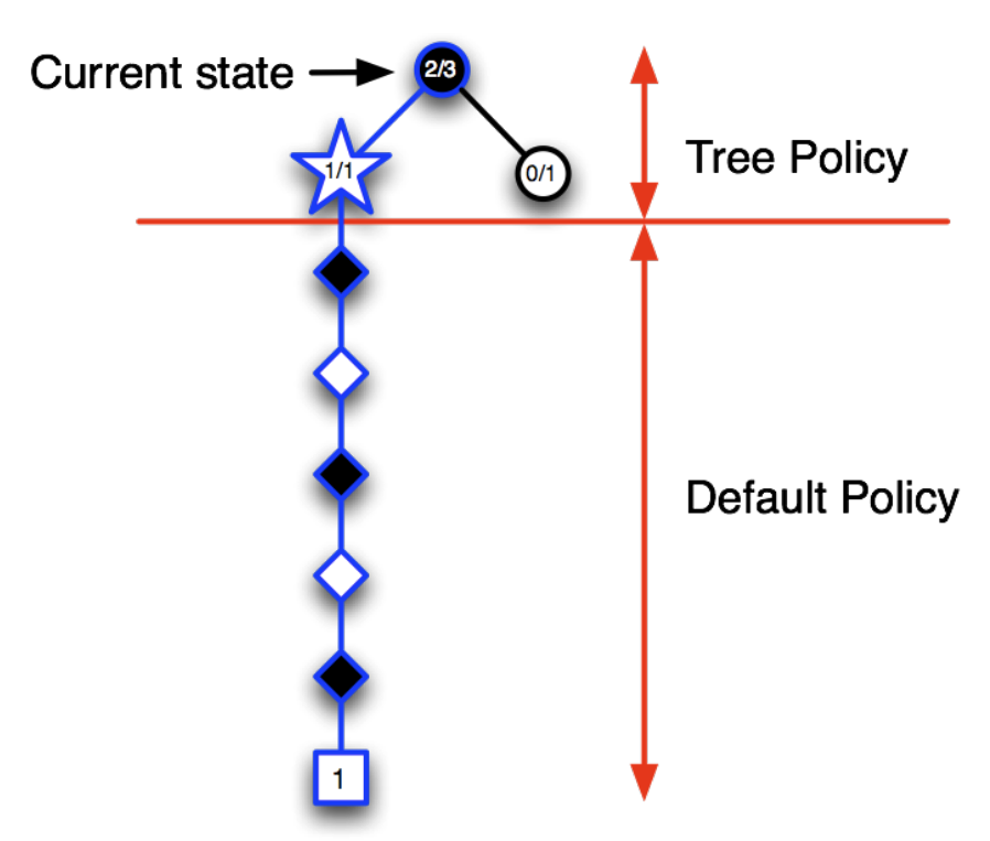
The tree policy now starts to guide us in the process of generating trajectories of experience and we proceed by taking an action that previously lead us to win the game. As it turns out, we lost a game again and update all the values in the search tree accordingly.

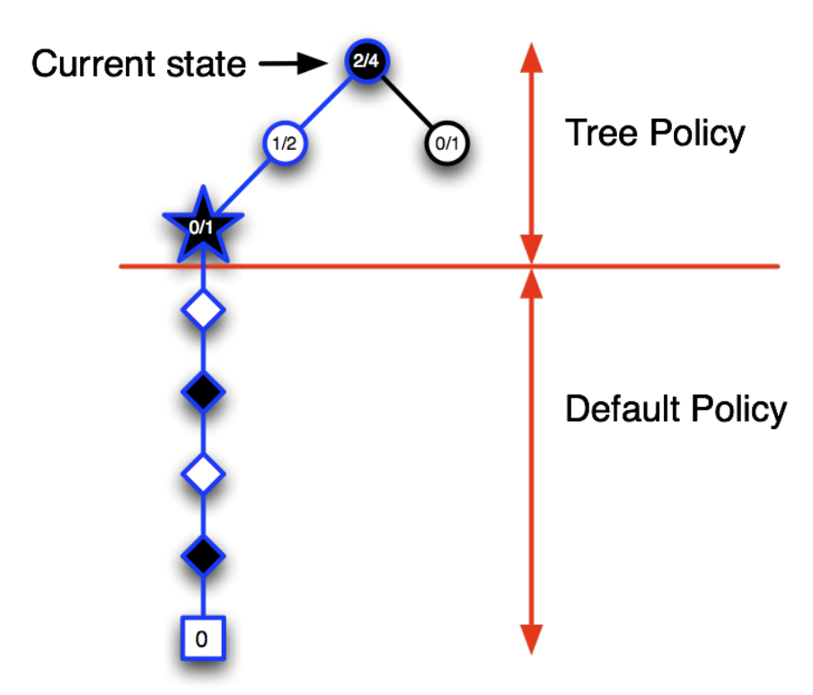
Finally, we take another action and add it to the search tree while updating all the relevant state-action pairs.

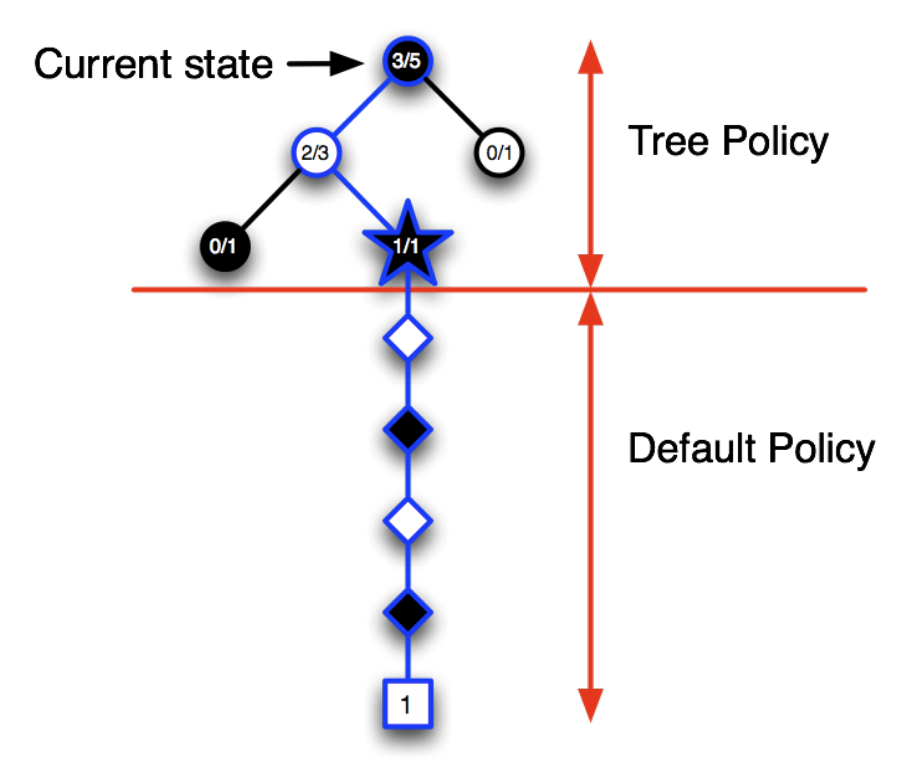
There are certain advantages associated with MC tree search algorithm:

• it is highly selective best-first search. This means that more promising actions are given high priority and explored in more depth than other actions.
• evaluates states dynamically (unlike dynamic programming, for example). This means that we spend time only on evaluating the current position and do not waste any time on looking into positions that are irrelevant.
• uses sampling to break the curse of dimensionality
• works for “black-box” models as it only requires samples
• computationally efficient

Temporal-Difference Search

Monte-Carlo tree search algorithm is just one example of a family of effective search algorithms. As we mentioned previously, the key ideas are forward search and sampling. MC tree search applies MC control to sub-MDPs from the current state. TD search, on the other hand, applies SARSA to sub-MDPs from the current state. As in model-free paradigm, there are certain benefits associated with using TD techniques.

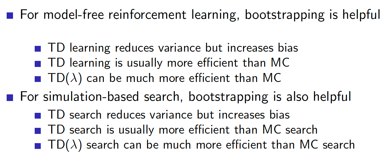
TD search works in a very similar fashion as MC tree search. We simulate episodes of experience from the current state $s_t$. For each step of simulation, we update state-action values by SARSA. The actions are selected based on the estimated $Q(s,a)$.

Note that for both MC tree search and TD search, we can use function approximators.

Dyna-2

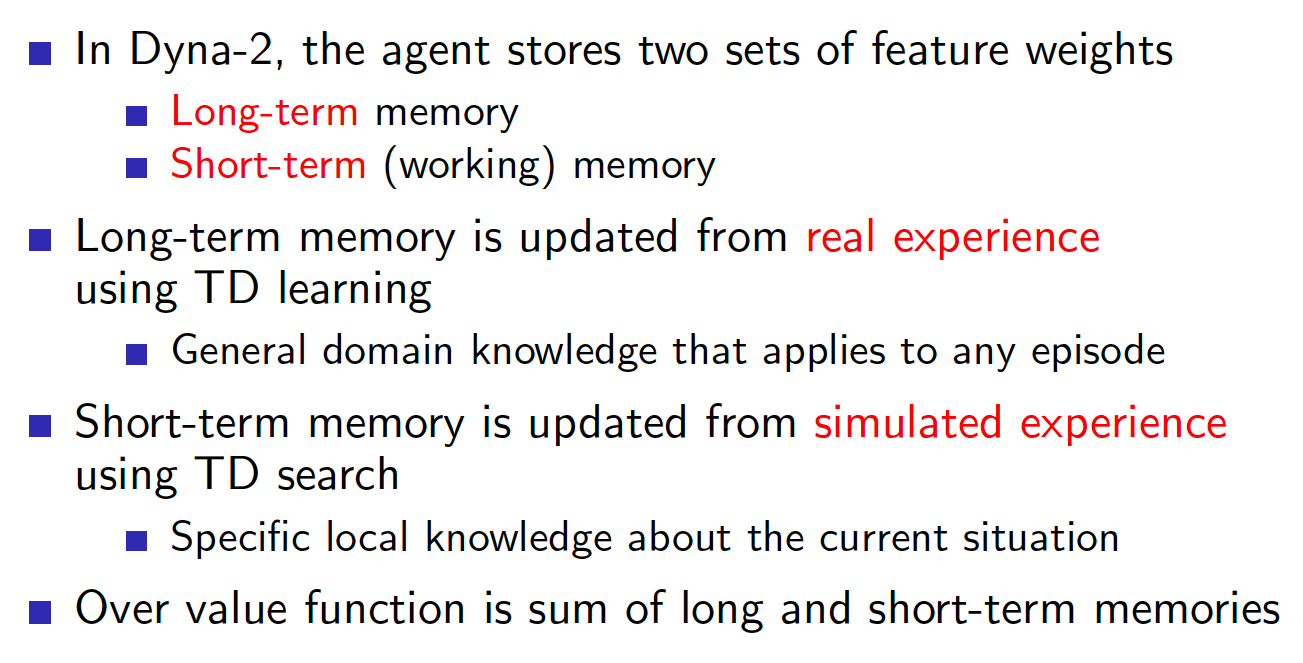
The graph below shows the relative performance of different algorithms applied to the game of Go. Strikingly, TD leaning performs very poorly. However, if we apply forward search, performance improves significantly!

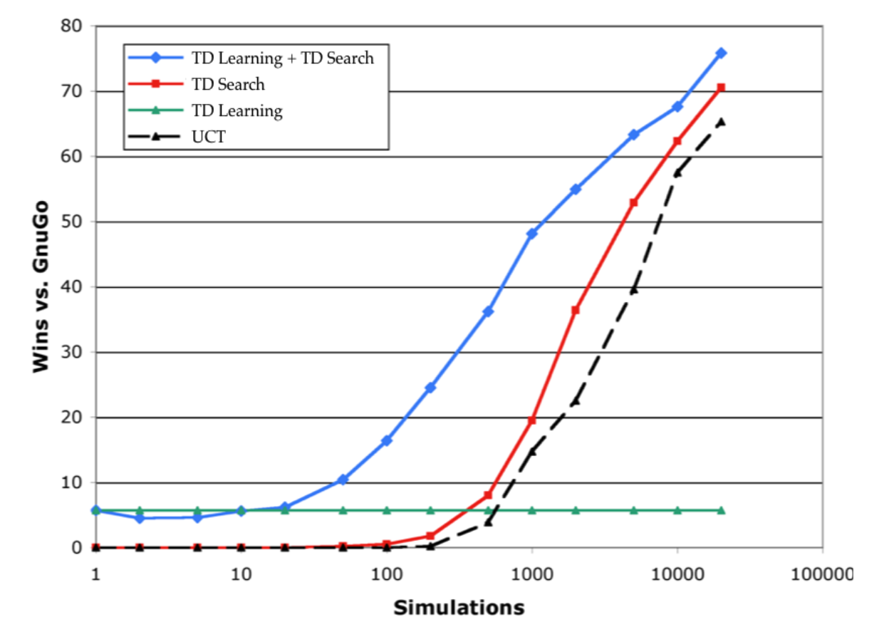
Exploration and Exploitation

There is always a trade-off in online decision making between exploration and exploitation. It is common that an overall optimal strategy requires that we sacrifice some immediate rewards to get higher rewards in the long-run. For that reason, we should always explore to find such strategies. Unlike supervised learning where we are given a dataset of “experience”, in RL our own actions determine what kind of data we are using for learning. This means that if we do not explore, the amount of data and its richness will be limited.

The key principles:

• Naive exploration. This is the simplest and most common approach to the exploration-exploitation dilemma. Basically, we take a random action with some small probability $\epsilon$.
• Optimistic initialization. The idea here is to initially assign quite optimistic values to state-action pairs, for example. During training, as agent explores the environment and receives lower rewards than what were initially assumed, he will be more willing to take the actions that have not been taken yet but still have higher values initially assigned to them.
• Optimism in the face of uncertainty. The idea here is that actions with more uncertain values should be preferred. For example, if our agent learned that taking action 1 is associated with a value of 10 but the value of taking action 2 is between 5 and 15, he should be more willing to take action 2.
• Probability matching. This means selecting actions according to probability that they are best.
• Information state search - lookahead search incorporating value of information.

There is also a distinction between state-action exploration and parameter exploration which is not often touched. State-action exploration is what is usually meant by exploration, i.e. it is about exploring state and action spaces. Parameter exploration, on the other hand, is more about exploring how we can parametrize our policy in PG methods, for example, or the structure of function approximator used in Q-learning algorithms.

The Multi-Armed Bandit

Multi-armed bandits are a common setup in the study of exploration and exploitation trade-off. Mathematically, multi-armed bandits are a tuple $<A, R>$, where $A$ is a known set of $m$ actions and

\[R^a(r) = P \left[R=r|A=a\right]\]

is an unknown probability distribution over rewards. At each time step $t$, an agent gets to choose an action $A_t \in A$ and the environment generates a reward $R_t \sim R^{a_t}$. The ultimate goal of the agent is to maximize the total reward, i.e.

\[\begin{equation*} \sum_{i=1}^{t}R_t. \end{equation*}\]

The value of action $a$, $q(a)$, is just the mean reward for this action, i.e.

\[\begin{equation*} q(a) = E\left[R|A=a\right]. \end{equation*}\]

The optimal value $v^*$ is the value of taking the action that yields the highest reward,

\[\begin{equation*} q^* = \max_{a\in A}q(a). \end{equation*}\]

We define regret as opportunity cost of not taking the optimal action $a^*$,

\[\begin{equation*} I_t = E\left[v^* - q(A_t)\right]. \end{equation*}\]

Naturally, the total regret is the total opportunity cost, i.e.

\[\begin{equation*} L_t = E \left[\sum_{i=1}^{t}v^* - q(A_i)\right]. \end{equation*}\]

Under this formulation, the problem of maximizing rewards is equivalent to the problem of minimizing the total regret. Let $N_t(a)$ represent the number of times action $a$ is taken up and including time $t$. Let $\Delta_a$ be the difference in value between action $a$ and the optimal action $a^*$, i.e.

\[\begin{equation*} \Delta_a = v^* - q(a). \end{equation*}\]

We can equivalently represent the total regret in the following way

\[\begin{align*} L_t = \sum_{a \in A}E\left[N_t(a) * \Delta_a\right]. \end{align*}\]

A good algorithm is the one that tends to choose fewer actions with big gaps and more actions with smaller gaps. Note that we do not know these gaps.

For most naive approaches to exploration, regret is a linear function of time (as shown on the graph below). For the greedy algorithm, the total regret is increasing linearly with time. This is explained by the fact that the greedy algorithm may get stuck by choosing a suboptimal action due to absence of exploration (for example, the algorithm was run for some time and learned/approximated q-values using MC approach. Due to high variance of the MC approach, it may be that a suboptimal action appears to have the highest q-value and is thus chosen by the agent forever).

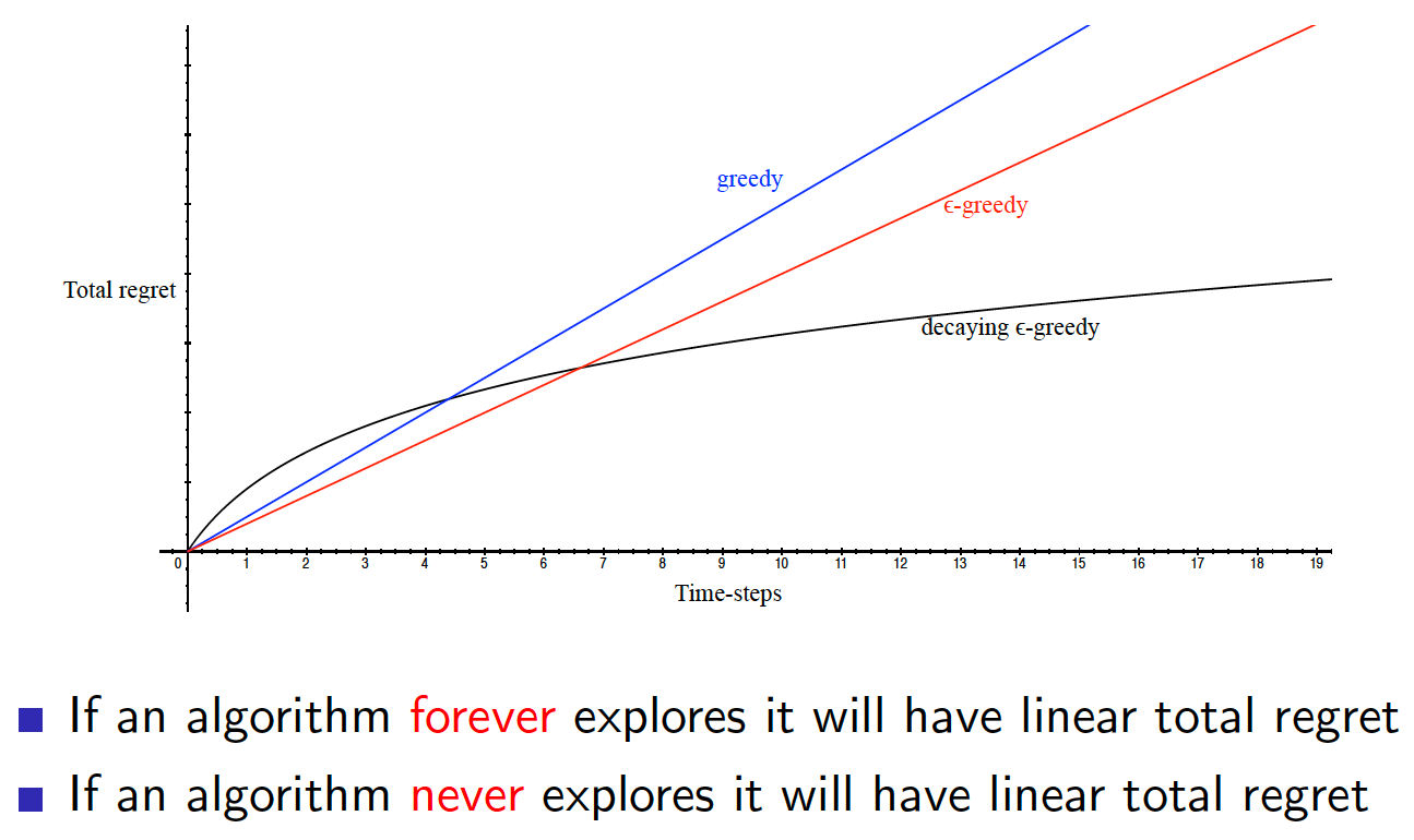
In the case of $\epsilon$-greedy algorithm, having a fixed probability $\epsilon$ of taking a random action ensures a minimum regret.

\[\begin{equation*} I_t = \frac{\epsilon}{A}\sum_{a \in A}\Delta_a. \end{equation*}\]

Finally, the decaying $\epsilon$-greedy algorithm has logarithmic asymptotic total regret. However, one needs to be careful about coming up with the decaying schedule.

The following theorem by Lai and Robbins puts a lower bound on the total asymptotic regret, i.e. such level of total regret that no algorithm can beat.

Theorem (Lai and Robbins): Asymptotic total regret is at least logarithmic in number of steps

\[\begin{equation*} \lim_{t\rightarrow \infty} L_t \ge \ln t \sum_{a|\Delta_a > 0}\frac{\Delta_a}{KL\left(R^a||R^{a^*}\right)}. \end{equation*}\]

Optimistic Initialization

The core idea is to assume that each action is very good (has a high value assigned to it) until proven otherwise and to act greedily with respect to action values. This encourages exploration early on in the training. Note that there is still no guarantee that we will not get stuck in some suboptimal action. This is because we may get “unlucky” and the rewards received from taking the optimal action may be low and thus discourage our agent to take it ever again. As a result, greedy policy combined with optimistic initialization still has linear total regret (same applies to $\epsilon$-greedy policy). In practice, optimistic initialization is still a very good approach that is hard to beat in certain domains.

Optimism in the Face of Uncertainty

Suppose we have a bandit problem with three arms: blue, red and green. The following graph shows our current beliefs about the worth of each of the three arms (probably after trying each arms for a number of times).

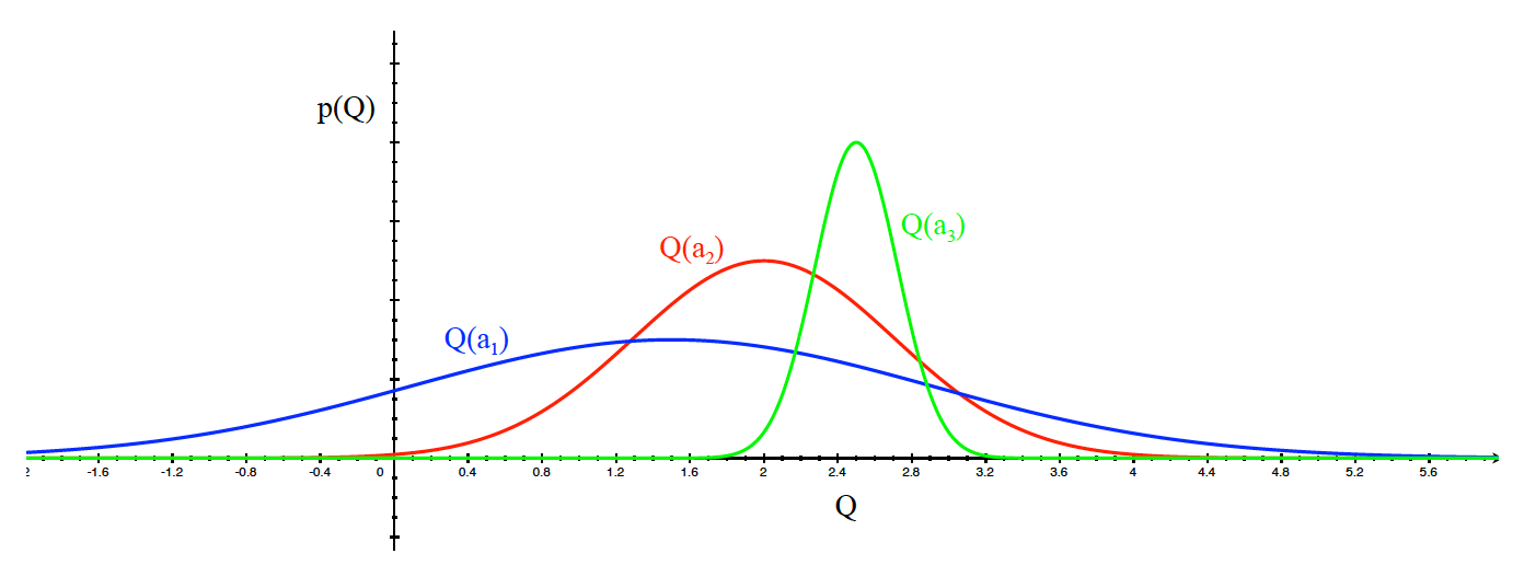
Which action should our agent take? The green arm is currently believed to have the highest expected q-value. A greedy policy might choose to exploit the green arm in this case. However, if we follow the optimism in the face of uncertainty principle, our agent should be willing to try those actions that have the highest potential to be optimal. In the current example, it would be the blue arm. This is because this arm has more weight in the range of higher q-values, i.e. right tail of the distribution (see the graph). As the agent takes more of the blue arm, the distribution of the q-value for this arm will shrink reflecting a higher certainty that we now have in its true worth. The updated graph may look something like below.

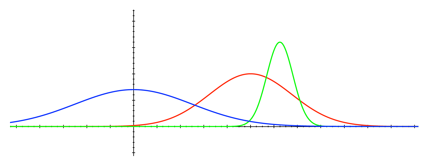
To formalize our approach, we can estimate an upper confidence $U_t(a)$ for each action value such that

\[\begin{equation*} q(a) \le Q_t(a) + U_t(a) \end{equation*}\]

with high probability, i.e. the probability that the true q-value is smaller than the sum of the mean of our current estimate of the true q-value and this upper confidence level is high. This upper confidence should depend on $N_t(a)$ - the number of times action $a$ was taken up to and including time $t$. The higher the $N_t(a)$, the lower the $U_t(a)$ should be as we have more confidence in our current estimate of the true q-value. As we explored action $a$ long enough, $U_t(a)$ should be approaching 0. Our policy is then to select those actions that maximize the Upper Confidence Bound (UCB)

\[\begin{equation*} A_t = \underset{a \in A}{argmax}Q_t(a) + U_t(a). \end{equation*}\]

How do we choose appropriate level of $U_t(a)$? We will make use of Hoeffding’s Inequality.

Theorem (Hoeffding’s Inequality) Let $X_1, X_2, \cdots, X_t$ be i.i.d. random variables taking values in $[0,1]$, and let $\bar{X}_t$ be the sample mean. Then

\[\begin{equation} P\left[E\left[X\right] > \bar{X}_t + u\right] \le e^{-2tu^2}. \label{eq:hoeffding} \end{equation}\]

In the context of the bandit problem, the Hoeffding’s inequality can be applied to get the following inequality

\[\begin{equation*} P\left[q(a) > Q_t(a) + U_t(a)\right] \le e^{-2 N_t(a)U_t(a)^2}. \end{equation*}\]

We can now fix some probability $p$, e.g. 95%, and find out the level of the $U_t(a)$ as follows

\[\begin{align*} p &= e^{-2 N_t(a)U_t(a)^2} \\ \ln(p) &= -2 N_t(a)U_t(a)^2 \\ U_t(a)^2 &= -\frac{\ln(p)}{2 N_t(a)} \\ U_t(a) &= \sqrt{-\frac{\ln(p)}{2 N_t(a)}}. \end{align*}\]

As we get more information, we should reduce the probability $p$. For example, we could set $p = t^{-4}$. This gives rise to the UCB1 algorithm.

\[\begin{equation} A_t = \underset{a \in A}{argmax}Q(a) + \sqrt{-\frac{\ln(p)}{2 N_t(a)}}. \end{equation}\]

In summary, the UCB1 algorithm was derived using the Hoeffding’s inequality. However, there are many other extensions that are based on other inequalities:

• Bernstein’s inequality
• Empirical Bernstein’s inequality
• Chernoff inequality
• Azuma’s inequality
• etc.

Bayesian Bandits

The UCB approach we discussed is general in the sense that it does not make any distributional assumptions of the reward function $R$. On the other hand, we could use Bayesian approach. Under the Bayesian approach, we utilize the prior knowledge of the distribution over action-value function. For example, consider a probability distribution $P\left[Q|w\right]$ over action-value function that is parametrized by $w$. If we assume Gaussian distributions, $w$ can be a vector of means and variances for each of the $k$ actions, i.e.

\[\begin{equation*} w = \left[\mu_1, \sigma_1^2, \mu_2, \sigma_2^2, \cdots, \mu_k, \sigma_k^2\right]. \end{equation*}\]

As an example, the graph below reflects our current believes about the actual q-values associated with each of the three arms.

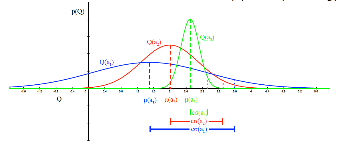
Bayesian methods compute the posterior distributions over $w$ as we gain more information from experience. These posterior distributions can then be utilized to guide our exploration. In particular, we could either implement upper confidence bounds or probability matching techniques. The former approach is the same that as UCB1 algorithm but we estimate the upper bound by adding $c$ standard deviations to the mean of the posterior distribution (as shown on the graph above). The policy is then to choose that action $a$ that maximizes $Q_t(a) + c\sigma(a)$.

Probability matching techniques, on the other hand, selects actions according to their respective probabilities of being the optimal action. As such, the probability of taking action $a$ is estimated as

\[\begin{equation*} \pi(a) = P\left[Q(a) = \max_{a'}Q(a')|R1, R2, \cdots, R_{t-1}\right]. \end{equation*}\]

In practice, one of the ways to implement probability matching is via Thompson sampling. We start by estimating the posterior distribution using the Bayes law. We then proceed by sampling $Q(a)$ from the posterior distribution. We select that action $a$ for which the drawn $Q(a)$ is highest. As it turns out, Thompson sampling achieves Lai and Robbins lower bound of total regret (for Bernoulli bandits).

In summary, Bayesian methods are as good as the prior information available.

Information State Search

Information state search is yet another idea in the exploration vs exploitation dilemma. To get the idea behind this concept, let us state the obvious fact that the reason we explore the environment is to gain information. If we have the perfect knowledge of q-values for each arm in the bandit problem, there is no need for us to explore and incur additional regret. Since information is valuable, can we assign a value to obtaining information? In other words, is there a way for us to quantify how much reward a decision-maker would be prepared to pay in order to obtain this information? If we find a way, it would mean that we can find an optimal way to trade exploitation for exploration. Obviously, we expect the price of information to be higher in uncertain situations. Hence, information state search should also be “optimistic in the face of uncertainty”.

Recall that we stated the multi-arm bandit problem as a single-step decision-making problem which is a tuple $<A, R>$. However, we could augment our problem statement by incorporating an information state $\tilde{S}_t$ that reflects all the information obtained up to time $t$, and a transition probability $\tilde{P}$. The later reflects the probability of moving from state $\tilde{s}$ to state $\tilde{s’}$ by taking action $a$. The augmented problem can then be considered as an MDP, i.e.

\[\begin{equation*} \tilde{M} = <\tilde{S}, A, \tilde{P}, R, \gamma>. \end{equation*}\]

The resulting MDP is an infinite MDP over information states. This MDP can be solved using reinforcement learning:

• Model-free RL
• Bayesian model-based RL. For example, Gittins indices (Gittins, 1979). This approach is known as Bayes-adaptive RL. It finds Bayes-optimal exploration/exploitation trade-off making use of prior distributions.

Example: Bayes-Adaptive RL

As an example, consider a Bernoulli bandit. In this setting, taking an action $a$ gives a reward of 1 with probability $\mu_a$ and a reward of 0 with probability $1 - \mu_a$. The information state $\tilde{s}$ is

\[\begin{equation*} \tilde{s} = <\alpha, \beta>, \end{equation*}\]

where $\alpha_a$ is the number of times action $a$ was taken and a reward of 0 was received, and $\beta_a$ is the number of times taking action $a$ resulted in a reward of 1. The graph below summarizes the approach.

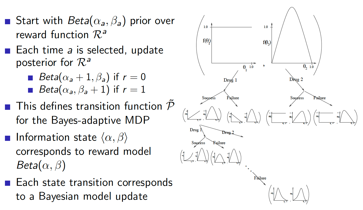
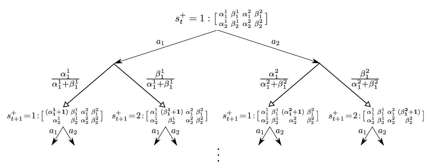
Bayes-adaptive MDP can be solved using dynamic programming and the solution to this MDP is known as Gittins index.

Contextual Bandits

Contextual bandits are an extension to simple multi-armed bandits. In particular, we add a state space. So contextual bandit is a tuple $<A, S, R>$. As usual, the goal is to maximize the cumulative reward.

UCB using Linear Regression

Let us use a linear combination of features to approximate the state-action function, i.e.

\[\begin{equation*} Q_{\theta}(s,a) = \phi(s,a)^T \theta \approx Q(s,a). \end{equation*}\]

Once we obtain the data, i.e. states and rewards over time, the parameters can be directly estimated by least squares regression. In particular,

\[\begin{align*} A_t &= \sum_{i=1}^t \phi(s_i, a_i)\phi(s_i, a_i)^T \\ b_t &= \sum_{i=1}^t \phi(s_i, a_i)r_i \\ \theta_t &= A_t^{-1}b_t. \end{align*}\]

The least squares regression estimates the mean action value. However, we can also estimate the corresponding variance.

\[\begin{equation*} \sigma_{\theta}^2(s,a) = \phi(s,a)^TA^{-1}\phi(s,a). \end{equation*}\]

We can then act in the environment by choosing that action $a$ that maximizes the upper confidence bound, i.e.

\[\begin{equation*} a_t = \underset{a \in A}{argmax}Q_{\theta}(s_t, a) + c \sqrt{\phi(s_t,a)^T A_t^{-1}\phi(s_t,a)}, \end{equation*}\]

where $c$ is some constant (representing the number of standard deviations from the mean). The UCB approach has an appealing geometric interpretation to it as well (see graph below).

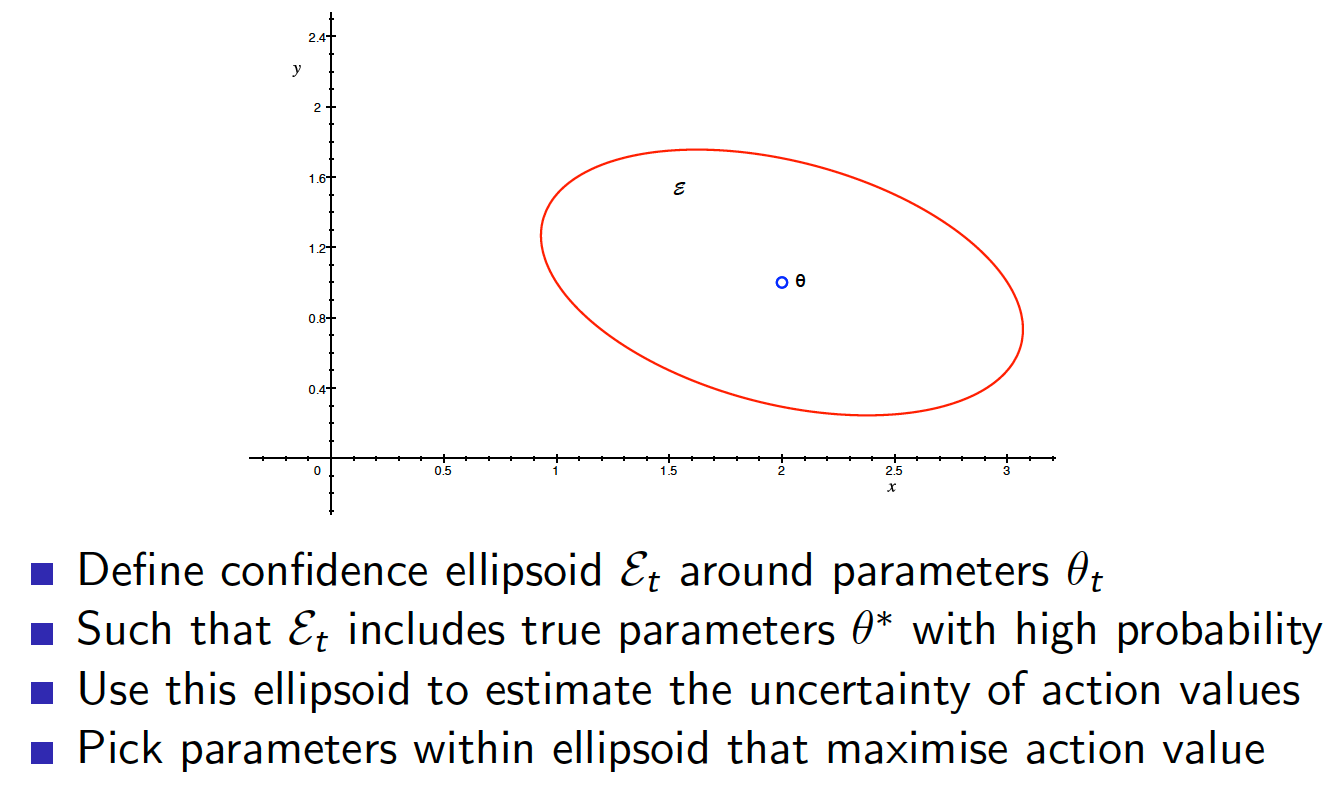
MDPs

All the principles developed in the bandit setting can be applied in MDPs albeit with some modifications. In summary, we covered the following approaches:

• naive exploration
• optimistic initialization
• optimism in the face of uncertainty
• probability matching
• information state search

Classic Games

There are many reasons why we study classic games and test our RL algorithms on them. Some of them are:

• games have simple rules but represent deep concepts
• classic games have been studied by humans for thousands of years which means there is a lot of human expertise to rely upon and benchmark against
• classic games are microcosms that encapsulate real world issues

The table below shows the level of performance that was achieved by AI (in general, not only RL) in classic games. Note that the table lists only the first program to achieve the mentioned level of performance in each domain.

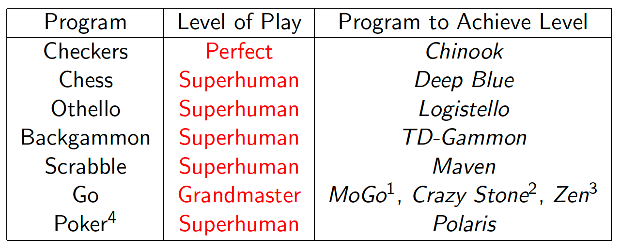
The table below shows a similar type of information but for RL algorithms only.

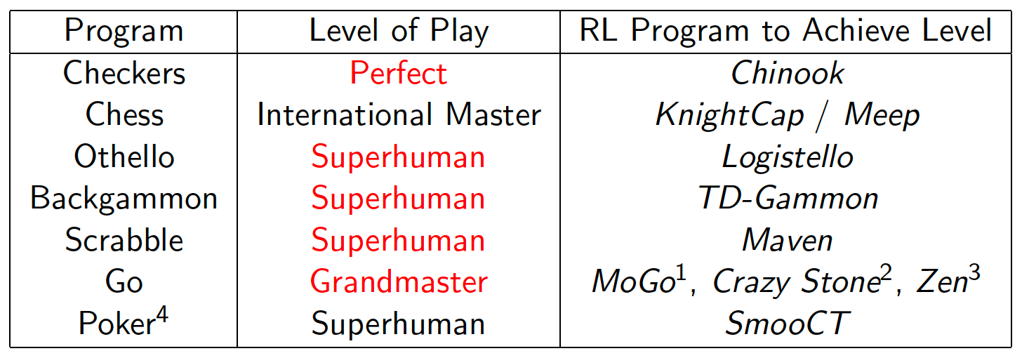
Game Theory

This section introduces some basic ideas from game theory.

Optimality in Games

In an MPD setting, an optimal policy for an agent is clear, i.e. he wants to maximize the sum of future discounted rewards by interacting with the environment. However, in games, there are usually more than one player. What is the optimal policy $\pi^i$ for ith player in this setting? If we fix the policies of other players $\pi^{-i}$, the best response $\pi_*^i(\pi^{-i})$ is the optimal policy for agent $i$ against these fixed policies. In other words, we can treat other players’ actions as part of the environment that agent $i$ interacts with. Now, since every player is going to improve his policy by playing in the environment against other players, we need to somehow define the overall optimal policy for all players. To do that, we introduce the concept of Nash equilibrium. More precisely, Nash equilibrium is a joint policy for all players, i.e. for each player $i$

\[\begin{equation} \pi^i = \pi_*^i(\pi^{-i}). \end{equation}\]

According to Wikipedia, “If each player has chosen a strategy—an action plan choosing its own action based on what it has seen happen so far in the game—and no player can increase its own expected payoff by changing its strategy while the other players keep theirs unchanged, then the current set of strategy choices constitutes a Nash equilibrium.” For example, in the game of rock paper scissors, the Nash equilibrium is achieved when every player plays rock/paper/scissors uniformly at random. In this equilibrium point, there is no expected change in reward for any player by changing his strategy. If some player decides to deviate from this equilibrium point, other player will be willing to exploit and change their policies to take advantage of that.

Single Agent and Self-Play RL

Best response strategy $\pi_*^i(\pi^{-i})$ is the solution to a single-agent RL problem. In other words, we treat other players as part of the environment. The whole game setting is then transformed to an MPD which can be tackled using the methods we developed previously. Best response strategy is then the solution of this MDP.

Nash equilibrium is a more powerful concept of optimality as it tells us the optimal way to behave among a set of different joint policies that the agents can adopt. How can Nash equilibrium be achieved in RL setting? As it turns out, Nash equilibrium is a fixed point of self-play RL. What this means is that instead of fixing the policies of other players in the environment and solving the resulting MDP for a single agent, we control all agents and let them play against each other. We allow each agent to improve their policies in response to the environment and actions generated by the opposing players. As a result, each player learns best responses to other players and one player’s policy determines another player’s environment (all players are adapting to each other, i.e. as one player get better, the other player have to adapt and improve on their policies to compete). If we ever achieve a fixed point in this process, that is no player is improving his current policy any further, we achieved the Nash equilibrium. Note that achieving this fixed point is no easy task and not all RL algorithms converge to this equilibrium point.

Two-Player Zero-Sum Games

A two-player zero-sum game, as the name implies, is a game between two players (player 1 is white and player 2 is black, by convention) that has equal and opposite rewards for the two players, i.e.

\[\begin{equation*} R^1 + R^2 = 0. \end{equation*}\]

The two common approaches to finding the Nash equilibrium in this kind of games are:

• game tree search (i.e. planning)
• self-play RL

Perfect and Imperfect Information Games

There are two types of games depending on availability of information. The first type is perfect information games (also known as Markov games). In this type of games, all information is available to the players, i.e. no hidden states (this also includes some games that include dice). For example, chess, checkers, Go, etc. On the opposite side, we have imperfect information games. By analogy, not all information about the state of the environment is revealed to the players. Examples of imperfect information games are poker and scrabble.

Minimax Search

Consider ourselves dealing with a two-player zero-sum game. Let us define a value function as follows

\[\begin{equation} v_{\pi}(s) = E_{\pi}\left[G_t|S_t=s\right], \label{eq:value_func} \end{equation}\]

where $\pi = <\pi^1, \pi^2>$. In other words, the value function represents the expected total reward for player 1 given joint policies, i.e. if player 1 continues to behave according to policy $\pi^1$ and player two continues to follow policy $\pi^2$. In two-player zero-sum games, it is common that there are no rewards until the game is finished and the winner get a reward of 1 and the loser gets a reward of -1 (by definition, the sum of rewards for the two players should be equal to 0). Thus, we only need to estimate the value function for player 1 as the value function of player 2 is going to be the opposite. In this case, Eq. ($\ref{eq:value_func}$) can be interpreted as the probability of either side winning the game starting in state $s$. For example, if $v_{\pi}(s) = 0$, there is a 50-50% chance that either side will win starting from state $s$ and following policies $\pi^1$ and $\pi^2$.

A minimax value function maximizes player 1 expected return under policy $\pi^1$ while minimizing player 1 expected return under policy $\pi^2$ (remember that player 2 is interested in player 1 getting a lower return as his return is the opposite of player 1 return), i.e.

\[\begin{equation} v_*(s) = \max_{\pi^1}\min_{\pi^2}v_{\pi}(s). \label{eq:minimax} \end{equation}\]

Again, as was the case in single-agent MDPs, if we know the minimax value function, we are done. We know what the optimal action for each player is in any given state $s$. The minimax function tells us who is going to win if both players are taking the optimal actions (player 1 maximizing the expected total reward and player 2 minimizing the expected total reward). As it turns out, in two-player zero-sum games with perfect information, there is a unique minimax value function and a minimax policy (that can be derived from the minimax value function) is a Nash equilibrium.

Minimax search is a way to estimate minimax values by constructing a search tree. The following example demonstrates how to estimate the minimax values. We start from a root node (state) and create a tree by taking all possible actions in each node (in this example, each player can take two actions in each state). We observe what the terminal rewards are (positive values are good for player 1 and negative values are good for player 2, i.e. we can think of rewards as only applying to player 1). For example, a possible game consisting of a sequence of moves ${a_1, b_1, a_1}$, where $a$ actions are taken by player 1 and $b$ actions are taken by player 2, resulted in a total reward of +7.

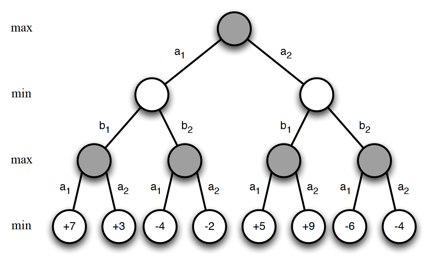
We proceed by updating the values of the preceding layers. Since the actions that lead to the terminal state are taken by player 1, the values of the nodes in the preceding layer are chosen as the maximum values of the terminal states (player 1 get to choose a move that finished the game). The results are as on the following graph.

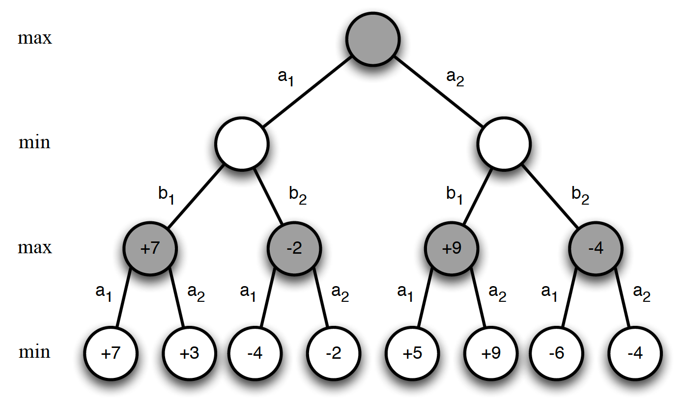
The actions that lead to the third layer are taken by player 2. This means that we use the minimum values of the nodes in the third layer to update the values of the nodes in the second layer. We get

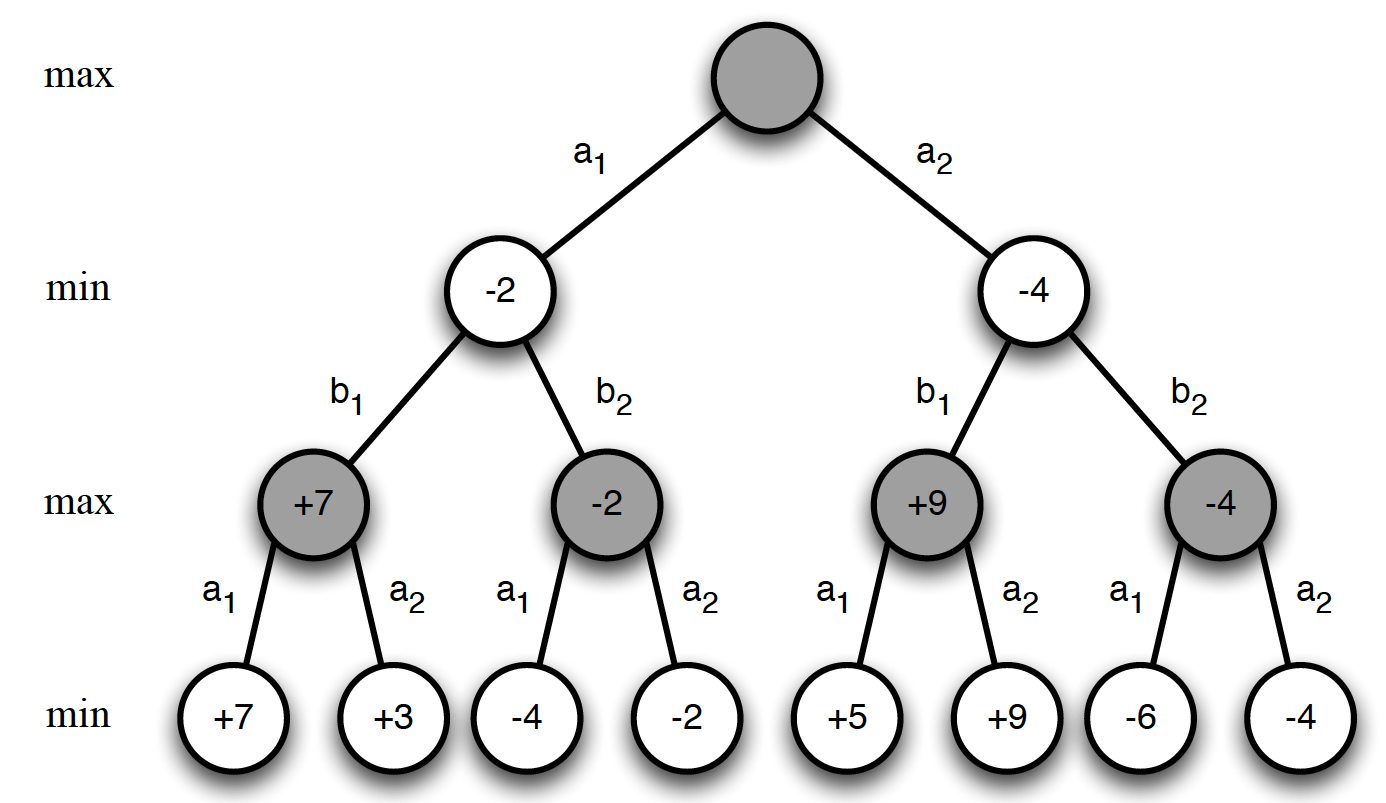
Finally,

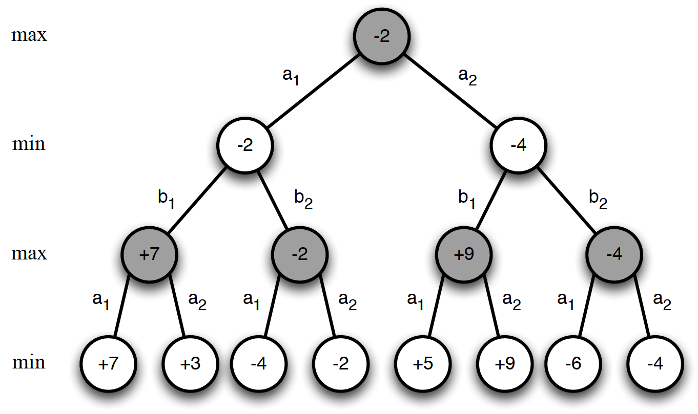
We also observe that knowing the minimax function gives us the optimal policies for both players. As such, the optimal way to play this game is for player 1 to take action $a_1$ on step 1, player 2 to take action $b_2$ on step 2 and player 1 take action $a_2$ on step 3. All three nodes have the same value. If any player deviates from this policy, the other player can exploit this to get a higher reward. For example, if player 2 chooses action $b_1$ on step 2 instead of action $b_2$, player 1 will choose action $a_1$ and get a reward of +7.

Value Function Approximator in Minimax Search

There are certain obvious disadvantages with this the minimax search algorithm:

• the search tree grows exponentially. Alpha-beta pruning algorithm is a search algorithm that seeks to decrease the number of nodes that are evaluated by the minimax algorithm.
• for most games, it is impractical to search to the end of the game

In view of these limitations, in practice, people use value function approximators $v(s,w) \approx v_*(s)$ (also known as evaluation functions and heuristic functions) and limit the number of steps that are taken to construct a search tree, e.g. we decide to look ahead only $n$ steps.

As an example, let us consider a binary-linear value function as applied to the game of chess. A binary feature vector $x(s)$ is a vector of 0’s and 1’s and represents presence or absence of certain chess pieces on the board (for current position $s$). Weight vector $w$ contains information on values of chess pieces. We can then evaluate any given position as

\[\begin{equation*} v(s, w) = x(s) \cdot w^T. \end{equation*}\]

The diagram below shows an example.

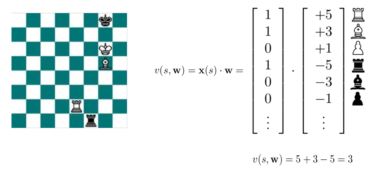
The value of the position is equal to 3 because white has a rook (a value of 5) and a bishop (a value of 3) against black’s rook (a value of -5). Remember that we estimate a value only from the perspective of player 1. We can then consider a possible game continuation by looking a number of steps ahead and creating a search tree. The game will then continue where player 1 chooses those actions (chess moves) from the created search tree that lead to states (chess positions) with higher values, while black will choose actions that lead to states with lower values.

The example we provided has a very simple representation of the value function for such a complex game as chess but it can be improved significantly if we included the positions of the pieces on the board in our feature vector and the corresponding values for these positions in the weight vector. In practice, there are many ways in which we can improve this binary-linear value function. The following picture summarizes what was used in Deep Blue chess program that defeated Garry Kasparov.

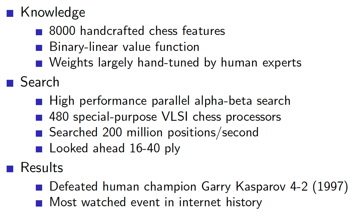
In summary, there is no RL as such in the minimax search approach that we discussed so far.

Self-Play TD Learning

Can the known techniques of RL be applied in the self-play setting? Fortunately, the answer is yes. Usually, there are no major changes that need to be applied to an RL algorithm for it to be successfully used in the self-play setting. However, instead of estimating the standard value function, we are estimating the minimax value function. Also, when we improve the policy, we improve it for both players. For example, we let both players act greedily with respect to the estimated minimax value function.

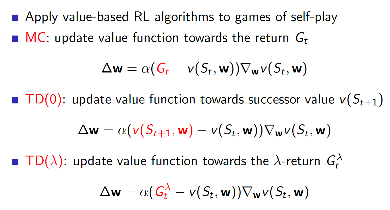
Policy Improvement with Afterstates

For deterministic games with known rules, it is enough for us to estimate $v_*(s)$, i.e. the minimax function (this means that we are not tied to the q-value as in model-free environment where state-transition function is not known to us). This is because we know exactly in what successor state we will end up after taking any given action. The optimal q-value in the current state $s$ is just the optimal minimax value function of the successor state.

\[\begin{equation*} q_*(s,a) = v_*(succ(s,a)), \end{equation*}\]

where $succ(s,a)$ is the successor state to state $s$ after taking action $a$. The corresponding policies for player 1 and player 2 are

\[\begin{align*} \text{Player 1}: A_t = \underset{a \in A}{argmax} \hspace{2mm} v_*(succ(S_t,a)) \\ \text{Player 2}: A_t = \underset{a \in A}{argmin} \hspace{2mm} v_*(succ(S_t,a)). \end{align*}\]

TD Gammon Example

This is one of the most successful applications of non-linear function approximators to classic games. TD Gammon used the following board representation that was fed to a neural network with a single hidden layer.

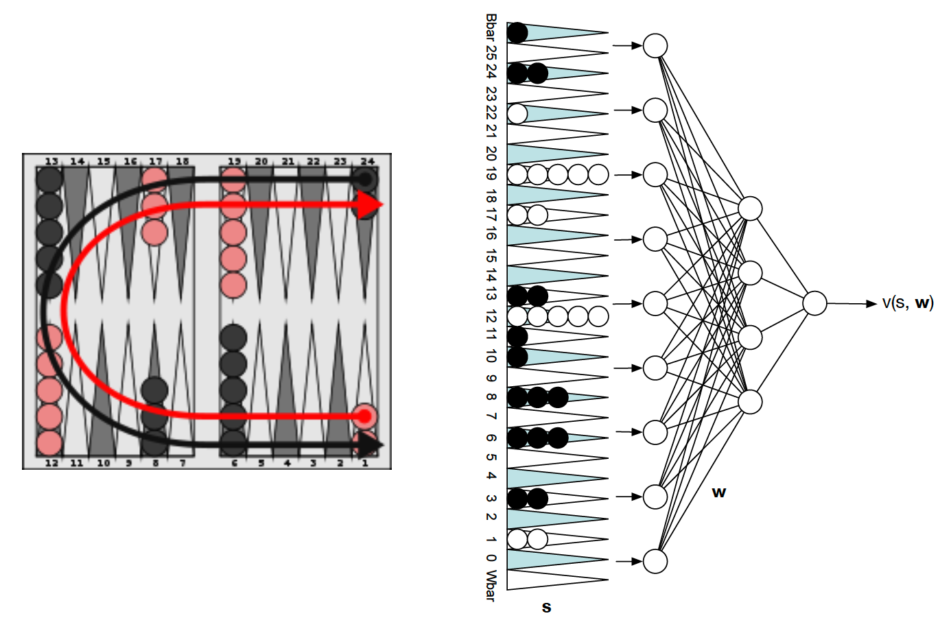
The model was initialized with random weights (no expert features were manually introduced) and learned the minimax value function completely via self-play. It used TD learning for adjusting its parameters.

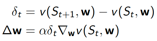
Interestingly, the model used exclusively greedy policy improvement without any exploration and always converged in practice. However, this is not true for most of other games. The reason why this approach worked so well for backgammon is that there is an inherent randomness introduced by dice. This means that, first, the inherent randomness allows the agent to explore the state-action space quite well. Secondly, this randomness smooths the minimax value function. In other words, it is quite hard for any player to execute a precise tactical sequence as it all depends on what the dice will turn out to be. In completely deterministic games, like chess and checkers, the minimax value function is not going to be smooth as there are precise tactical sequences and a single move can mean a difference between a winning and a losing position (recall that neural networks are implicitly assuming that similar inputs are producing similar outputs).

Combining RL with Minimax Search

So far we considered the minimax search and self-play RL separately. Is there a way for us to combine the two approaches/algorithms to improve our agents?

Simple TD

The most obvious approach is to first learn the minimax value function via games of self-play and then use this value function in minimax search, i.e.

\[\begin{equation*} v_+(S_t, w) = \underset{s \in leaves(S_t)}{minimax} \hspace{2mm} v(s,w). \end{equation*}\]

The graph below shows the results that have been achieved in the classic games domain using this simple approach.

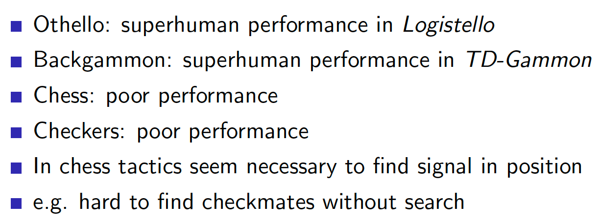
While this approach is simple and may be applicable to certain games, this is not the best way to combine the two algorithms. This is because the minimax search is applied to an already learned minimax value function and does actually help us in learning the minimax value function in the first place. The natural question is: Can we utilize minimax search in helping us learn a better minimax value function?

TD Root

The idea in TD root is to use the minimax algorithm to improve the way we learn the minimax value function. We update our current value estimate for some root state $s$ by using the successor search value. Instead of updating our current value estimate towards the estimate at the successor state, we take an action and run a minimax search algorithm from $succ(s,a)$. We then update the value of the root state $s$ towards the minimax value of the terminal node (terminal node can be the end of the game or a specified $n$ steps away from the root node). The diagram below demonstrates the principle.

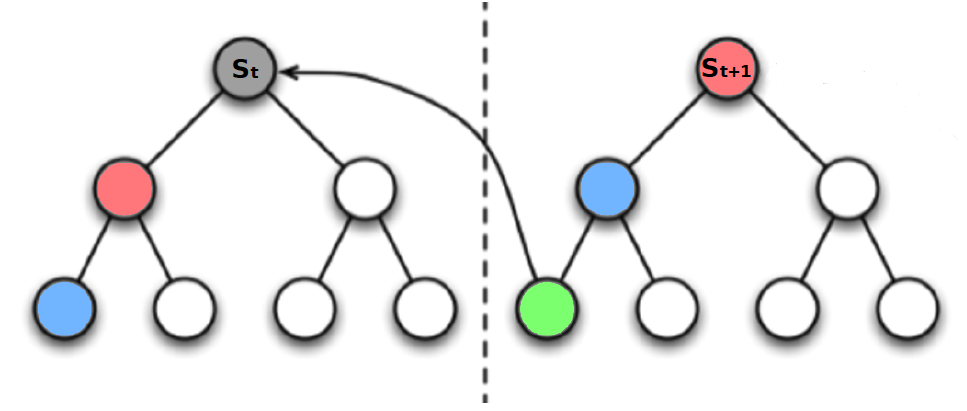
Let us explain what is going on on the diagram. We start from root node $s$. We take some action according to our current policy and end up in state $s_{t+1}$. From $s_{t+1}$ we run a minimax search either until the end of the game or for a specified depth. Suppose that the minimax search lead us to the green node. We then use the value at this green node as our TD target.

TD Leaf

TD root is a naive approach that can easily be improved upon. TD leaf is one possible extension. The idea of TD leaf is to update the value of the terminal leaf of the current minimax search (starting from state $s$) using the value of the terminal leaf of the minimax search of the successor leaf $s_{t+1}$. The diagram below explains the concept.

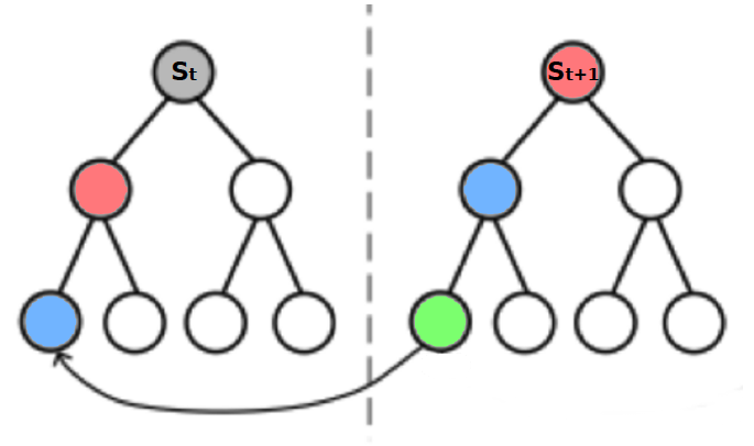
We start in state $s$ and run a minimax search that ends up in the blue leaf. Thus, the value of the blue leaf determines the values of all the nodes visited on the way from state $s$ to the blue leaf (including the value of the successor red leaf). We proceed by taking an action that leads us to the red successor state $s_{t+1}$ and run a minimax search from this state. Suppose we end up in some terminal state (green node). Now, it means that the value of red node should be updated to the value of the green node, not the blue node as was the case previously. However, instead of updating the value of the red node towards green node, it is enough for us to update the value of the blue node towards green node. In subsequent games, when we perform the minimax search from state $s$, the updated values of the leaf nodes may lead us to a different terminal leaf node (which is more correct now).

TD leaf algorithm has really been successful in chess and checkers.

TreeStrap

The idea of TreeStrap method is to run a big search tree from current state $s$ and then use the information obtained from the whole tree to update the value function for all the intermediate nodes and the root node. Unlike TD root and TD leaf, we are not discarding valuable information by running a whole search and only updating a value for a single node (state).

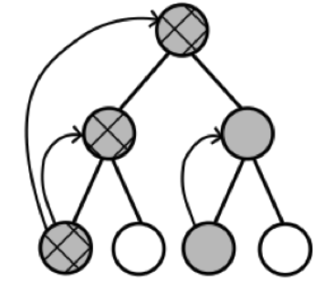
Simulation-Based Search

As a reminder, the idea of simulation-based approach in model-based RL was to generate experience from the current state using the learned model of the environment and apply the techniques of model-free RL to find the optimal way to behave. The same idea can be applied in the case of self-play RL. In particular, we let agents simulate games of self-play from root state and then apply model-free RL techniques to the simulated experience. Using Monte-Carlo approach, we get Monte-Carlo Tree Search (MCTS) algorithm. The most effective variant of MCTS is UCT algorithm that uses the Upper Confidence Bound (UCB) algorithm in each node of the tree to balance exploration and exploitation (see lecture 9 for details). Self-play UCT converges on minimax values.

Note that MCTS algorithm is best performing method in many challenging games.

Imperfect Information Games

If you take MCTS or UCT algorithms that work quite well in perfect information games, they will diverge in imperfect information settings. A very effective and recent algorithm for imperfect information games is Smooth UCT Search.

Recipe for Successful RL in Games

The following key ideas are most likely responsible for successful RL implementations in classic games:

• binary input features
• binary-linear value function
• self-play, i.e. not playing against a fixed opponent but rather against an evolving opponent
• search is crucial